Slicing Return Distributions: A Practical Route to Multivariate Distributional RL
An informal walkthrough of multivariate distributional reinforcement learning with sliced divergences: why projection-based objectives help, and why one-sample TD still matters.
Welcome! This is a more informal walkthrough of our ICML 2026 paper, Multivariate Distributional Reinforcement Learning Using Sliced Divergences. The paper has the formal definitions, theorems, and proofs. Here I want to tell the story more directly: what breaks when distributional RL moves beyond scalar returns, why slicing is a useful trick, and where the annoying but important TD subtlety shows up.
The short version is this: sliced divergences let us compare multivariate return distributions by looking at many one-dimensional projections. That gives a practical way to reuse familiar one-dimensional objectives, but it does not make every problem disappear. In particular, the objective still has to behave well with the one-sample Bellman bootstrapping used in standard TD.
Table of contents
- Why multivariate distributional RL?
- What makes the multivariate case awkward?
- The slicing trick
- Which one-dimensional divergence should we slice?
- From sliced divergences to a TD update
- Uniform slicing vs max slicing
- What the theory says
- The TD sampling catch
- Experiments
- Practical takeaway
- Open question
- Bibliography
Why multivariate distributional RL?
Distributional RL usually starts from a simple question: instead of learning only the expected return, why not learn the full return distribution? In the scalar case, this means modelling a random return such as
$$ Z^\pi(s,a) = \sum_{t=0}^{\infty} \gamma^t R_t. $$
That perspective has been very useful in scalar-reward RL. But many objects we may want to predict are not scalar. Rewards can be vector-valued. Returns can correspond to several objectives or several horizons. Successor features also naturally predict a vector of discounted feature occupancies rather than a single number. In value-gradient or Sobolev-style TD, the objects of interest can also be coupled through richer, structured targets.
So the paper asks the next question: what if the return itself lives in $\mathbb R^d$?
A convenient way to write the multivariate return is
$$ Z^\pi(s,a) = \sum_{t=0}^{\infty} \left( \prod_{k=1}^{t} \Gamma(S_k,A_k) \right) R_t, \qquad R_t \in \mathbb R^d. $$
Here $\Gamma(s,a)$ may be as simple as $\gamma I_d$, but it may also be a matrix. The corresponding distributional Bellman update is
$$ (\mathcal T^\pi Z)(s,a) \stackrel{D}{=} R(s,a) + \Gamma(s,a) Z(S',A'). $$
The goal is not merely to predict each component independently. The goal is to model the joint return law: correlations, shape, and higher-order structure included.
What makes the multivariate case awkward?
Why not just take scalar distributional RL and add dimensions? Because many of the convenient scalar tricks are secretly one-dimensional.
Categorical grids are manageable in one dimension, but grow combinatorially in $d$. Quantile parameterizations are powerful in scalar distributional RL, but there is no equally simple multivariate ordering. Wasserstein distances are conceptually natural, and in one dimension they are efficient because they reduce to sorting samples. In higher dimensions, exact empirical optimal transport can become much more expensive.
A useful contrast is:
| Problem | Typical empirical cost |
|---|---|
| 1D Wasserstein by sorting | $\mathcal O(n \log n)$ |
| exact multivariate OT | often around $\mathcal O(n^3 \log n)$ |
That is a pretty brutal jump. The paper’s motivation is not “Wasserstein is bad.” Quite the opposite: Wasserstein gives a very clean contraction story in some settings. The problem is that exact multivariate Wasserstein is often too expensive and statistically unfriendly for the kind of particle-based TD update we want to run.
The slicing trick
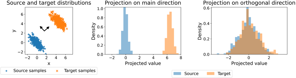
The core trick is to avoid comparing high-dimensional distributions directly. Instead, look at them from many one-dimensional directions.
Take a direction on the unit sphere,
$$ \theta \in \mathbb S^{d-1}, $$
and project a vector $x \in \mathbb R^d$ by
$$ P_\theta(x) = \langle \theta, x \rangle. $$
If $\mu$ and $\nu$ are two laws on $\mathbb R^d$, then $(P_\theta)_\#\mu$ and $(P_\theta)_\#\nu$ are now one-dimensional laws. We can compare those with any one-dimensional divergence $\Delta$.
Uniform slicing averages these one-dimensional comparisons over directions:
$$ \mathbf S\Delta_p^p(\mu,\nu) = \int_{\mathbb S^{d-1}} \Delta^p\!\left((P_\theta)_\#\mu, (P_\theta)_\#\nu\right) \, d\sigma(\theta). $$
In practice, we approximate the integral with random directions:
$$ \widehat{\mathbf S\Delta}_p^p(\mu,\nu) = \frac{1}{L}\sum_{\ell=1}^{L} \Delta^p\!\left((P_{\theta_\ell})_\#\mu, (P_{\theta_\ell})_\#\nu\right), \qquad \theta_\ell \sim \mathrm{Unif}(\mathbb S^{d-1}). $$
This is the main practical move: lift tractable one-dimensional divergences to multivariate return distributions via projections.
Which one-dimensional divergence should we slice?
Once everything is projected to one dimension, we can reuse familiar base divergences. The paper focuses mostly on three families.
Wasserstein. This is the natural baseline. In one dimension, $\mathbf W_p$ can be estimated by sorting projected samples, so the sliced estimator is cheap per direction. But Wasserstein has an important issue for one-sample TD: its sample gradients can be biased relative to the population objective.
Cramér. In one dimension, the Cramér distance is an $L_2$ distance between CDFs:
$$ \mathbf C_2(\mu,\nu) = \ell_2^2(\mu,\nu) = \int_{\mathbb R} |F_\mu(u)-F_\nu(u)|^2\,du. $$
The sliced Cramér objective is therefore
$$ \mathbf{SC}_2^2(\mu,\nu) = \int_{\mathbb S^{d-1}} \ell_2^2\!\left((P_\theta)_\#\mu,(P_\theta)_\#\nu\right)\,d\sigma(\theta). $$
This ends up being the safest practical default in the paper: efficient, projection-based, and compatible with the usual one-sample TD setting.
MMD. Maximum Mean Discrepancy compares probability laws through a kernel. Its squared form is
$$ \mathbf{MMD}_k^2(\mu,\nu) = \mathbb E_{x,x'\sim\mu}[k(x,x')] + \mathbb E_{y,y'\sim\nu}[k(y,y')] -2\mathbb E_{x\sim\mu,y\sim\nu}[k(x,y)]. $$
Sliced MMD applies the same idea after projection. It is a useful alternative, especially because squared MMD-style objectives can satisfy the sample-gradient property we care about later.
| Base divergence | Why it is attractive | Main caveat |
|---|---|---|
| Wasserstein | natural geometry; cheap in 1D | biased sample gradients for standard TD |
| Cramér | CDF distance; TD-friendly | less common than Wasserstein |
| MMD | kernel-based moment matching | kernel choice matters |
From sliced divergences to a TD update
How does this become an RL update?
We use a particle critic. For a state-action pair $(s,a)$, the critic predicts particles
$$ \{z_i\}_{i=1}^{N} = \{Z_\phi(s,a,i)\}_{i=1}^{N}. $$
Given a sampled transition $(s,a,r,s')$ and next action $a'\sim\pi(\cdot\mid s')$, the target particles are
$$ \{\hat z_i\}_{i=1}^{N} = \{r + \Gamma(s,a) Z_{\phi^-}(s',a',i)\}_{i=1}^{N}. $$
Then we minimize a sliced divergence between predicted and target particles.
A clean pseudocode version is:
sample transition (s, a, r, s')
sample next action a' ~ pi(. | s')

for i = 1,...,N:
    z_i     = Z_phi(s, a, i)
    zhat_i  = r + Gamma(s,a) Z_phi_minus(s', a', i)

draw projection directions theta_1,...,theta_L
project z_i and zhat_i on each theta_l
compute the 1D divergence on each projection
average over directions
update phi by gradient descent
That is the distributional TD update, but with a multivariate return law and a sliced objective.
Uniform slicing vs max slicing
Uniform slicing averages random views. Max slicing asks for the most discriminative view:
$$ \mathbf{MS}\Delta(\mu,\nu) = \sup_{\theta\in\mathbb S^{d-1}} \Delta\!\left((P_\theta)_\#\mu,(P_\theta)_\#\nu\right). $$
This is a very tempting idea. If random directions miss the interesting discrepancy, max slicing tries to find it.
But the tradeoff is important:
| Variant | Intuition | Strength | Weakness |
|---|---|---|---|
| uniform slicing | average many random views | simple, parallel, preserves TD suitability when the base objective has it | can miss discriminative directions if too few projections are used |
| max slicing | search for the strongest view | gives a norm-based contraction result for matrix-discounted updates | the maximizing direction depends on the sample and can break one-sample TD compatibility |
This tradeoff is basically the core tension of the paper.
What the theory says
I would not read the theory as a list of isolated theorems. The useful way to remember it is as a chain of answers.
Does slicing preserve metric structure?
Yes. If the base one-dimensional divergence $\Delta$ is a metric, then uniform slicing gives a metric on multivariate laws. Max slicing also preserves metricity under the same kind of assumption.
Do we get a Bellman contraction in the standard multivariate case?
Yes, for shared scalar discounting. If
$$ \Gamma(s,a)=\gamma I_d, $$
then uniform slicing inherits the univariate contraction factor. In the paper notation,
$$ \overline{\mathbf S\Delta_p}\big(\mathcal T^\pi\eta_1,\mathcal T^\pi\eta_2\big) \le c(\gamma)\, \overline{\mathbf S\Delta_p}(\eta_1,\eta_2). $$
What about dense or matrix discounting?
This is where things get less comfortable. For updates of the form
$$ R + \Gamma(s,a)Z(S',A'), $$
we may want a contraction that depends only on
$$ \bar L = \sup_{s,a}\|\Gamma(s,a)\|_{\mathrm{op}}. $$
Uniform slicing does not generally give that norm-only contraction. The paper shows negative results for uniform sliced divergences and for common MMD constructions.
Can max slicing recover that contraction?
Yes. Max slicing gives a way to recover a norm-only contraction under general matrix-discounted Bellman updates, assuming the base divergence satisfies the relevant one-dimensional conditions.
So why not always use max slicing?
Because contraction at the population level is not the whole story. Standard TD uses sampled Bellman targets, and max slicing can interact badly with that sampling.
The TD sampling catch
This is the part I find easiest to underestimate.
The true Bellman target is a mixture distribution. It averages over transition randomness and policy randomness:
$$ \mu = \mathbb E_{S',A'}\left[\mathrm{Law}\big(R + \Gamma Z(S',A')\big)\right]. $$
But in standard TD, we usually draw one successor and build a sampled Bellman target:
$$ \hat\mu = \mathrm{Law}\big(R + \Gamma Z(s',a')\big). $$
So training is not directly optimizing the full population objective. It is optimizing an expected sample loss. That is fine only when the sample gradients line up with the population gradient.
The property we want is
$$ \mathbb E_{X_{1:m}\sim\mu} \left[ \nabla_\phi \mathcal D(\hat\mu_m,\nu_\phi) \right] = \nabla_\phi \mathcal D(\mu,\nu_\phi). $$
The paper calls this the unbiased sample-gradient property.
This is where the practical recommendation comes from:
| Objective | One-sample TD suitability | Comment |
|---|---|---|
| sliced Cramér | good | strong default for distributional policy evaluation |
| sliced MMD-style objective | good when using the squared objective with the right estimator | viable alternative |
| sliced Wasserstein | problematic | attractive geometry, but biased sample gradients |
| max-sliced objectives | generally problematic | direction selection depends on the sample |
The annoying lesson is that an objective can have a nice population-level contraction story and still be a bad match for stochastic TD.
Experiments
The experiments are useful because they separate two questions that are easy to mix together:
- Does the critic learn the full return distribution accurately?
- Does the resulting agent get good control performance?
These are related, but not identical.
Chain environment.
The chain is a controlled policy-evaluation setup. It lets us compare standard one-sample TD with a near-exact TD variant where the transition-mixture target is explicitly constructed.
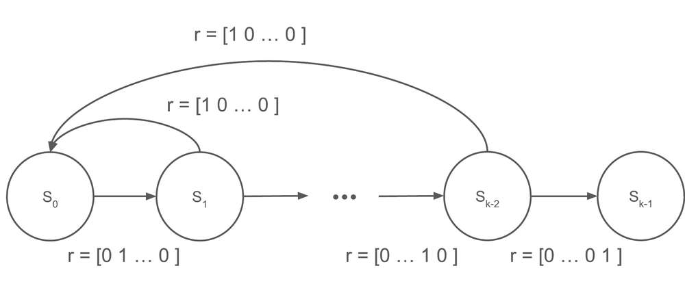
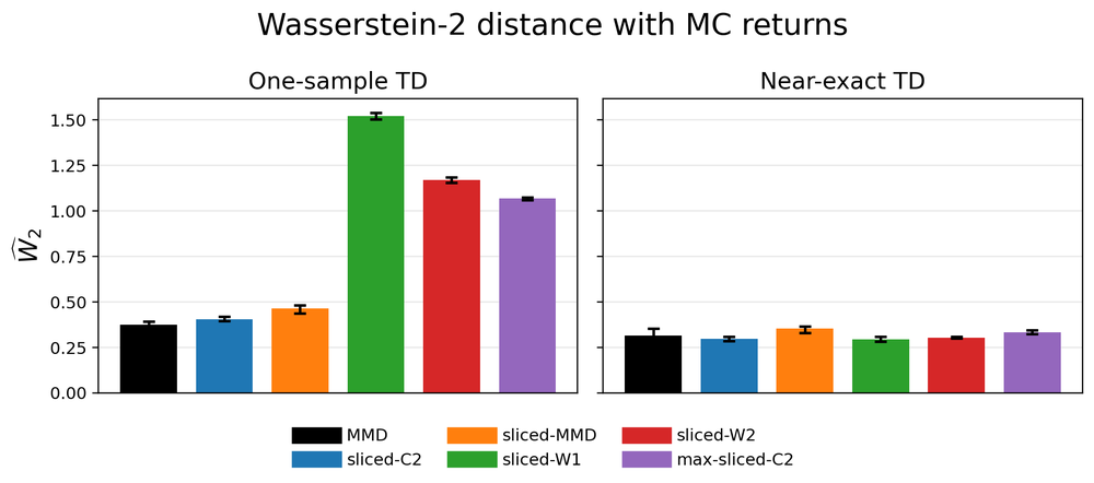
The result is exactly the story the theory predicts. When the target mixture is available, gradient bias matters less. Under ordinary one-sample TD, the objectives violating the unbiased sample-gradient property degrade substantially.
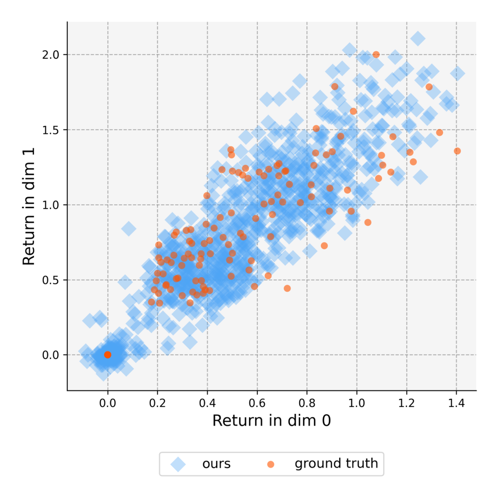
Maze from pixels.
The maze experiments move to pixel observations and vector-valued rewards. Here exact TD is not available, so this is closer to the training regime we actually care about.
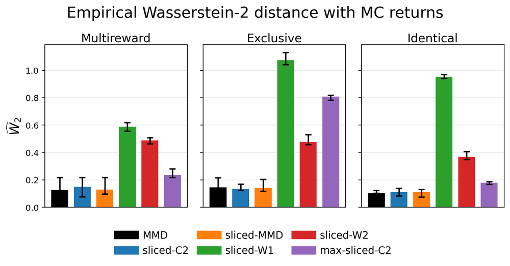
The qualitative plot is also helpful: Monte Carlo returns and critic particles are both clouds in return space. When sliced Cramér works, it is not merely getting the mean right; it is matching the shape of the return distribution.
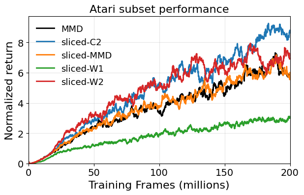
Atari control.
The Atari subset tells a slightly different story. Sliced Cramér performs strongly, but sliced Wasserstein can also work very well for control despite looking worse as a distributional matching objective in earlier experiments.
That is not a contradiction. Policy improvement depends heavily on expected return estimates. An objective can model the full return distribution poorly and still give useful expectations for control. For policy evaluation, that is not enough; for control, it may sometimes be enough.
Practical takeaway
If I had to compress the paper into one practical recommendation, it would be:
For multivariate distributional policy evaluation with standard one-sample TD, sliced Cramér is the safest default.
Sliced MMD is also viable. Sliced Wasserstein is worth testing for control, especially because its geometry is appealing and it can work empirically, but I would be more careful about treating it as a reliable distributional learning objective under one-sample TD. Max slicing is theoretically valuable for matrix-discounted Bellman operators, but its sample-dependent direction selection makes it delicate in stochastic TD.
Open question
The clean open question is whether we can get all of the following at once:
- norm-only contraction under general matrix discounts,
- compatibility with one-sample TD,
- tractable estimators,
- dimension-friendly statistical rates.
In paper notation, the dream is a divergence $\mathcal D$ such that
$$ \overline{\mathcal D}(\mathcal T^\pi\eta_1,\mathcal T^\pi\eta_2) \le c(\bar L)\,\overline{\mathcal D}(\eta_1,\eta_2), \qquad \bar L = \sup_{s,a}\|\Gamma(s,a)\|_{\mathrm{op}}, $$
while still behaving correctly when the Bellman target is sampled through the usual one-sample TD update.
That is the gap the paper leaves open.
Bibliography
A few references that are useful for reading the post:
- Bellemare, Dabney, and Munos, 2017. A Distributional Perspective on Reinforcement Learning.
- Bellemare, Danihelka, Dabney, Mohamed, Lakshminarayanan, Hoyer, and Munos, 2017. The Cramér Distance as a Solution to Biased Wasserstein Gradients.
- Dabney, Rowland, Bellemare, and Munos, 2018. Distributional Reinforcement Learning with Quantile Regression.
- Rowland, Dadashi, Kumar, Munos, Bellemare, and Dabney, 2019. Statistics and Samples in Distributional Reinforcement Learning.
- Zhang, Chen, Zhao, Xiong, Qin, and Liu, 2021. Distributional Reinforcement Learning for Multi-Dimensional Reward Functions.
- Wiltzer, Farebrother, Gretton, and Rowland, 2024. Foundations of Multivariate Distributional Reinforcement Learning.
- Rabin, Peyré, Delon, and Bernot, 2011; Bonneel, Rabin, Peyré, and Pfister, 2015; Nadjahi et al., 2020. Work on sliced Wasserstein and sliced probability divergences.
- Deshpande et al., 2019. Max-Sliced Wasserstein Distance and Its Use for GANs.
- Gretton, Borgwardt, Rasch, Schölkopf, and Smola, 2012. A Kernel Two-Sample Test.
- Nguyen-Tang, Gupta, and Venkatesh, 2021. Distributional Reinforcement Learning via Moment Matching.
- Killingberg and Langseth, 2023. The Multiquadric Kernel for Moment-Matching Distributional Reinforcement Learning.
- Barreto et al., 2017. Successor Features for Transfer in Reinforcement Learning.
- Debes and Tuytelaars, 2026. Distributional Value Gradients for Stochastic Environments.
- Gallici et al., 2024. Simplifying Deep Temporal Difference Learning.