Slicing Return Distributions: A Practical Route to Multivariate Distributional RL
Sliced divergences make multivariate return distributions tractable by reducing them to one-dimensional projections, but TD learning still depends on how the Bellman target is sampled from the environment.
Distributional RL replaces a scalar value target with a distribution over returns [1]. In the scalar case this is already useful: the critic can represent variability, skew, multimodality, and risk-sensitive information that an expectation collapses away. Rainbow also made distributional RL one of the main axes of improvement over DQN-style baselines [16]. In the multivariate case, the object being learned is richer again [5] [6]. A return can have several reward components, as in multi-objective RL benchmarks [17], or in Atari games whose primitive rewards admit a fixed decomposition into several sources [5]. It can also collect several horizons [18], successor-feature coordinates [14], or value-gradient/Sobolev targets [15] that couple values with derivative information.
The difficulty is that most of the convenient distributional-RL machinery is one-dimensional. Sorting samples gives cheap Wasserstein estimates in one dimension, CDF-based distances are easy to compute, and many theoretical arguments are written for scalar returns [3] [4]. Once returns live in $\mathbb R^d$, direct distribution comparison is no longer the cheap sorting problem used by many scalar DRL methods.
Sliced divergences make this comparison tractable by repeatedly reducing it to one-dimensional problems [7] [8] [9]. Project both multivariate laws onto a direction, compare the projected samples with a one-dimensional divergence, then aggregate over directions. This keeps the estimator close to the practical tools used in scalar distributional RL while still defining an objective on multivariate return distributions.
A separate issue comes from how TD targets are instantiated. In TD learning, the Bellman target is usually not the full transition-and-policy mixture. It is built from sampled environment transitions and sampled next actions. A distributional objective can behave well against the population Bellman operator and still give biased or unstable gradients under this one-sample TD procedure [2] [4]. This distinction is the main reason sliced Wasserstein, sliced Cramér, sliced MMD, uniform slicing, and max slicing do not play the same role.
Table of contents
- Why multivariate distributional RL?
- What makes the multivariate case awkward?
- The slicing trick
- Which one-dimensional divergence should we slice?
- From sliced divergences to a TD update
- Uniform slicing vs max slicing
- What the theory says
- The TD sampling catch
- Experiments
- Practical takeaway
- Open question
- Bibliography
Why multivariate distributional RL?
Distributional RL usually starts from a simple question: instead of learning only the expected return, why not learn the full return distribution [1]? In the scalar case, this means modelling a random return such as
$$ Z^\pi(s,a) = \sum_{t=0}^{\infty} \gamma^t R_t. $$
That perspective has been very useful in scalar-reward RL. But many objects we may want to predict are not scalar. Rewards can be vector-valued. In multi-objective RL, benchmarks explicitly expose several reward components, so the return naturally records trade-offs between objectives rather than one collapsed scalar [17]. The same idea appears in some Atari environments: their primitive rewards admit a fixed decomposition into multiple sources, which Zhang et al. use to model a joint distribution over source-specific returns [5]. Returns can also correspond to several horizons [18]. Successor features naturally predict a vector of discounted feature occupancies rather than a single number [14]. In value-gradient or Sobolev-style TD, the objects of interest can also couple value targets with derivative information [15].
So the paper asks the next question: what if the return itself lives in $\mathbb R^d$?
A convenient way to write the multivariate return is
$$ Z^\pi(s,a) = \sum_{t=0}^{\infty} \left( \prod_{k=1}^{t} \Gamma(S_k,A_k) \right) R_t, \qquad R_t \in \mathbb R^d. $$
Here $\Gamma(s,a)$ may be as simple as $\gamma I_d$, but it may also be a matrix. The corresponding distributional Bellman update is
$$ (\mathcal T^\pi Z)(s,a) \stackrel{D}{=} R(s,a) + \Gamma(s,a) Z(S',A'). $$
The goal is not merely to predict each component independently. The goal is to model the joint return law: correlations, multimodality, and dependencies between coordinates included.
What makes the multivariate case awkward?
Why is the multivariate case not just scalar distributional RL with a larger output layer? The difficulty is that several standard scalar parameterizations and losses rely on operations that are simple on the real line: fixed ordered supports, sorted samples, one-dimensional CDFs, and pairwise matching after sorting.
Categorical grids, as in C51, are manageable in one dimension [1], but grow combinatorially in $d$. Quantile parameterizations are powerful in scalar distributional RL [3], but they rely on an ordered real line; there is no equally simple ordering of multivariate samples. Wasserstein distances are also cheap in one dimension because empirical samples can be sorted before being matched. In higher dimensions, exact empirical optimal transport can become much more expensive [6].
A useful contrast is:
| Problem | Typical empirical cost |
|---|---|
| 1D Wasserstein by sorting | $\mathcal O(n \log n)$ |
| exact multivariate OT | often around $\mathcal O(n^3 \log n)$ |
That is a pretty brutal jump. The paper’s motivation is not “Wasserstein is bad.” Quite the opposite: Wasserstein gives a very clean contraction story in some settings. The problem is that exact multivariate Wasserstein is often too expensive and statistically unfriendly for the kind of particle-based TD update we want to run.
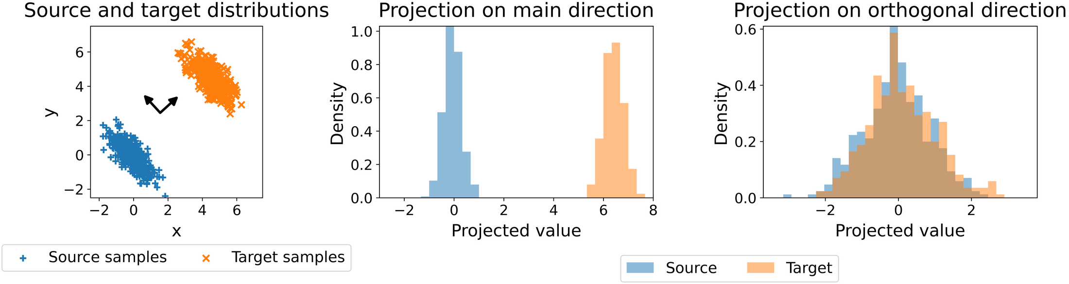
The slicing trick
The core trick is to avoid comparing high-dimensional distributions directly [7] [8] [9]. Instead, look at them from many one-dimensional directions.
Take a direction on the unit sphere,
$$ \theta \in \mathbb S^{d-1}, $$
and project a vector $x \in \mathbb R^d$ by
$$ P_\theta(x) = \langle \theta, x \rangle. $$
If $\mu$ and $\nu$ are two laws on $\mathbb R^d$, then $(P_\theta)_\#\mu$ and $(P_\theta)_\#\nu$ are now one-dimensional laws. We can compare those with any one-dimensional divergence $\Delta$.
Uniform slicing averages these one-dimensional comparisons over directions:
$$ \mathbf S\Delta_p^p(\mu,\nu) = \int_{\mathbb S^{d-1}} \Delta^p\!\left((P_\theta)_\#\mu, (P_\theta)_\#\nu\right) \, d\sigma(\theta). $$
In practice, we approximate the integral with random directions:
$$ \widehat{\mathbf S\Delta}_p^p(\mu,\nu) = \frac{1}{L}\sum_{\ell=1}^{L} \Delta^p\!\left((P_{\theta_\ell})_\#\mu, (P_{\theta_\ell})_\#\nu\right), \qquad \theta_\ell \sim \mathrm{Unif}(\mathbb S^{d-1}). $$
This is the main practical move: lift tractable one-dimensional divergences to multivariate return distributions via projections.
Which one-dimensional divergence should we slice?
Once everything is projected to one dimension, we can reuse familiar base divergences. The paper focuses mostly on three families.
Let
$$ \nu_z = \frac{1}{n}\sum_{i=1}^{n}\delta_{z_i}, \qquad \nu_{\hat z} = \frac{1}{n}\sum_{i=1}^{n}\delta_{\hat z_i} $$
be the empirical predicted and target particle distributions. For a projection direction $\theta$, write
$$ \nu_z^\theta = (P_\theta)_\#\nu_z, \qquad \nu_{\hat z}^\theta = (P_\theta)_\#\nu_{\hat z}. $$
Each sliced estimator is obtained by applying a one-dimensional estimator to $\nu_z^\theta$ and $\nu_{\hat z}^\theta$, then averaging over sampled directions.
Wasserstein. This is the natural baseline. In one dimension, $\mathbf W_p$ can be estimated by sorting projected samples. If $u_i=P_\theta z_i$ and $v_i=P_\theta \hat z_i$, and $u_{(i)}$, $v_{(i)}$ denote the sorted samples, then for equal sample sizes
$$ \widehat{\mathbf W}_{p}^{p}(\nu_z^\theta,\nu_{\hat z}^\theta) = \frac{1}{n}\sum_{i=1}^{n}|u_{(i)}-v_{(i)}|^p. $$
The sliced estimator averages this over $L$ directions:
$$ \widehat{\mathbf{SW}}_{p}^{p}(\nu_z,\nu_{\hat z}) = \frac{1}{L}\sum_{\ell=1}^{L} \widehat{\mathbf W}_{p}^{p}(\nu_z^{\theta_\ell},\nu_{\hat z}^{\theta_\ell}). $$
Sorting costs $\mathcal O(n\log n)$ per projection. The caveat is not the estimator itself, but one-sample TD: Wasserstein sample gradients can be biased relative to the population objective [2] [4].
Cramér. In one dimension, the Cramér distance is an $L_2$ distance between CDFs [2]:
$$ \mathbf C_2(\mu,\nu) = \ell_2^2(\mu,\nu) = \int_{\mathbb R} |F_\mu(t)-F_\nu(t)|^2\,dt. $$
Empirically, merge and sort the projected samples from both distributions. Between two consecutive sorted breakpoints $t_k$ and $t_{k+1}$, the empirical CDF difference is constant; call it $\Delta_k$. Then
$$ \widehat{\mathbf C}_2(\nu_z^\theta,\nu_{\hat z}^\theta) = \sum_{k=1}^{K-1}(t_{k+1}-t_k)\Delta_k^2. $$
The sliced Cramér objective is therefore estimated as
$$ \widehat{\mathbf{SC}}_2(\nu_z,\nu_{\hat z}) = \frac{1}{L}\sum_{\ell=1}^{L} \widehat{\mathbf C}_2(\nu_z^{\theta_\ell},\nu_{\hat z}^{\theta_\ell}). $$
This also costs $\mathcal O(n\log n)$ per projection because the main step is sorting. In the paper, this is the safest practical default: efficient, projection-based, and compatible with the usual one-sample TD setting.
MMD. Maximum Mean Discrepancy compares probability laws through a kernel [11]. Its squared form is
$$ \mathbf{MMD}_k^2(\mu,\nu) = \mathbb E_{x,x'\sim\mu}[k(x,x')] + \mathbb E_{y,y'\sim\nu}[k(y,y')] -2\mathbb E_{x\sim\mu,y\sim\nu}[k(x,y)]. $$
The empirical biased estimator on projected samples is
$$ \widehat{\mathbf{MMD}}_{k,b}^2 = \frac{1}{n^2}\sum_{i,j=1}^{n}k(u_i,u_j) + \frac{1}{n^2}\sum_{i,j=1}^{n}k(v_i,v_j) - \frac{2}{n^2}\sum_{i,j=1}^{n}k(u_i,v_j). $$
Sliced MMD applies the same idea after projection [9]:
$$ \widehat{\mathbf{SMMD}}_{k}^{2}(\nu_z,\nu_{\hat z}) = \frac{1}{L}\sum_{\ell=1}^{L} \widehat{\mathbf{MMD}}_{k,b}^{2}(\nu_z^{\theta_\ell},\nu_{\hat z}^{\theta_\ell}). $$
This costs $\mathcal O(n^2)$ per projection because all pairwise kernel evaluations are used. It is a useful alternative, especially because squared MMD-style objectives can satisfy the sample-gradient property we care about later [12] [13].
For one projection direction, the empirical estimators have the following costs:
| Divergence | Time complexity |
|---|---|
| Wasserstein $\mathbf W_p$ | $\mathcal O(n\log n)$ |
| Cramér $\mathbf C_2$ | $\mathcal O(n\log n)$ |
| MMD$_k$ | $\mathcal O(n^2)$ |
MMD is the natural kernel baseline here, not a new loss introduced by slicing. Nguyen-Tang, Gupta, and Venkatesh introduced MMD-style moment matching to distributional RL [12]. In the multivariate setting, Zhang et al. used MMD for multi-dimensional reward functions [5], and Wiltzer et al. analyze MMD-based multivariate distributional RL, including the restrictions needed for contraction results [6]. Sliced MMD keeps this baseline in the comparison, but applies the kernel loss after one-dimensional projections.
From sliced divergences to a TD update
How does this become an RL update?
We use a particle critic. For a state-action pair $(s,a)$, the critic predicts particles
$$ \{z_i\}_{i=1}^{N} = \{Z_\phi(s,a,i)\}_{i=1}^{N}. $$
Given a sampled transition $(s,a,r,s')$ and next action $a'\sim\pi(\cdot\mid s')$, the target particles are
$$ \{\hat z_i\}_{i=1}^{N} = \{r + \Gamma(s,a) Z_{\phi^-}(s',a',i)\}_{i=1}^{N}. $$
Then we minimize a sliced divergence between predicted and target particles.
A clean pseudocode version is:
sample transition (s, a, r, s')
sample next action a' ~ pi(. | s')

for i = 1,...,N:
    z_i     = Z_phi(s, a, i)
    zhat_i  = r + Gamma(s,a) Z_phi_minus(s', a', i)

draw projection directions theta_1,...,theta_L
project z_i and zhat_i on each theta_l
compute the 1D divergence on each projection
average over directions
update phi by gradient descent
That is the distributional TD update, but with a multivariate return law and a sliced objective.
Uniform slicing vs max slicing
Uniform slicing averages one-dimensional discrepancies over random projection directions. Max slicing replaces this aggregation with optimization over the most discriminative direction [10]:
$$ \mathbf{MS}\Delta(\mu,\nu) = \sup_{\theta\in\mathbb S^{d-1}} \Delta\!\left((P_\theta)_\#\mu,(P_\theta)_\#\nu\right). $$
Since the supremum is usually not available in closed form, it is approximated by optimizing the projection direction on the unit sphere. In the paper, this matters because max slicing is used to obtain contraction guarantees beyond the shared scalar-discount setting.
Uniform slicing and max slicing therefore answer different contraction questions. Uniform slicing gives the clean result for vector-valued returns with shared scalar discounting. Max slicing targets matrix-discounted Bellman updates, where the linear part is controlled through an operator-norm bound. The sample-based TD issue is separate and comes later.
What the theory says
The Bellman update in the paper is written with a matrix discount,
$$ (\mathcal T^\pi \eta)(s,a) := \mathrm{Law}\!\left(R(s,a)+\Gamma(s,a)X'\right), \qquad X'\sim \eta(S',A'). $$
The canonical cases are:
Classical distributional RL. The return is scalar,
$$ d=1, \qquad \Gamma(s,a)=\gamma\in[0,1). $$
Multivariate returns with shared scalar discount. The return is vector-valued, but every coordinate uses the same scalar discount,
$$ d>1, \qquad \Gamma(s,a)=\gamma I_d = \begin{pmatrix} \gamma & 0 & \cdots & 0\\ 0 & \gamma & \cdots & 0\\ \vdots & \vdots & \ddots & \vdots\\ 0 & 0 & \cdots & \gamma \end{pmatrix}. $$
This is the setting where uniform slicing gives the direct multivariate contraction result. If the base one-dimensional divergence satisfies the required translation, scaling, and mixture conditions, then
$$ \overline{\mathbf S\Delta_p}\big(\mathcal T^\pi\eta_1,\mathcal T^\pi\eta_2\big) \le c(\gamma)\, \overline{\mathbf S\Delta_p}(\eta_1,\eta_2). $$
Result #1 — standard case. For $\Gamma=\gamma I_d$, $\mathbf S\Delta_p$ inherits the contraction of the base one-dimensional divergence $\Delta$.
General constant matrix. The discount can be a fixed matrix,
$$ \Gamma(s,a)\equiv \Gamma, \qquad \Gamma\in\mathbb R^{d\times d}. $$
A simple example is a diagonal multi-horizon discount [18],
$$ \Gamma = \mathrm{diag}(\gamma_1,\ldots,\gamma_d) = \begin{pmatrix} \gamma_1 & 0 & \cdots & 0\\ 0 & \gamma_2 & \cdots & 0\\ \vdots & \vdots & \ddots & \vdots\\ 0 & 0 & \cdots & \gamma_d \end{pmatrix}. $$
State-action dependent matrix discount. The most general case considered in the paper allows
$$ \Gamma(s,a) = \begin{pmatrix} \gamma_{11}(s,a) & \gamma_{12}(s,a) & \cdots & \gamma_{1d}(s,a)\\ \gamma_{21}(s,a) & \gamma_{22}(s,a) & \cdots & \gamma_{2d}(s,a)\\ \vdots & \vdots & \ddots & \vdots\\ \gamma_{d1}(s,a) & \gamma_{d2}(s,a) & \cdots & \gamma_{dd}(s,a) \end{pmatrix}. $$
For matrix-discounted updates, the target contraction form is controlled by the operator norm,
$$ \bar L := \sup_{(s,a)\in\mathcal S\times\mathcal A} \|\Gamma(s,a)\|_{\mathrm{op}}, $$
and asks for
$$ \overline{\mathcal D}\big(\mathcal T^\pi\eta_1,\mathcal T^\pi\eta_2\big) \le c(\bar L)\, \overline{\mathcal D}(\eta_1,\eta_2). $$
Result #2 — dense case. For general matrix-discounted updates with $\bar L<1$, uniform sliced divergences do not generally satisfy the norm-based contraction criterion; common MMD constructions can fail it as well.
Max slicing replaces averaging over directions with optimization over the most discriminative direction:
$$ \mathbf{MS}\Delta(\mu,\nu) = \sup_{\theta\in\mathbb S^{d-1}} \Delta\!\left((P_\theta)_\#\mu,(P_\theta)_\#\nu\right). $$
Result #3 — max-slicing. Under the stated assumptions on the base divergence, max-slicing recovers the norm-based contraction form for matrix-discounted Bellman updates.
The TD sampling catch
For a divergence to lead to a working TD algorithm, population-level contraction is not enough. The stochastic update also needs sample-based gradients to agree, in expectation, with the gradient of the population objective.
The population Bellman target is a mixture law over transition and policy randomness:
$$ \mu = \mathbb E_{S',A'}\left[\mathrm{Law}\big(R + \Gamma Z(S',A')\big)\right]. $$
In standard TD, this mixture is usually instantiated from one sampled successor:
$$ \hat\mu = \mathrm{Law}\big(R + \Gamma Z(s',a')\big). $$
So the algorithm optimizes an expected sample loss. The required compatibility condition is
$$ \mathbb E_{X_{1:m}\sim\mu} \left[ \nabla_\phi \mathcal D(\hat\mu_m,\nu_\phi) \right] = \nabla_\phi \mathcal D(\mu,\nu_\phi). $$
This condition is the unbiased sample-gradient property: the plug-in gradient obtained from an empirical target should be unbiased for the gradient of the population loss. This is exactly the issue created by one-sample TD: the algorithm sees $\hat\mu$, but the distributional Bellman target is $\mu$.
Uniform slicing. If the powered one-dimensional base objective $\Delta^p$ has unbiased sample gradients, then the powered uniform sliced objective $\mathbf S\Delta_p^p$ also has unbiased sample gradients. Averaging over random directions does not add a new sample-selection step.
Max-slicing. Max-slicing does not have unbiased sample gradients in general. The maximizing direction is selected from the same empirical sample used to evaluate the loss, which creates selection bias even when every fixed direction would be fine.
Base objectives. Wasserstein has biased sample gradients in the one-sample TD regime. Squared Cramér / energy distance and squared MMD-style objectives avoid this issue, and uniform slicing preserves that property for the powered objective.
| Objective | Unbiased |
|---|---|
| $\mathbf{SW}_p$ | ✗ |
| $\mathbf{SC}_2^2$ | ✓ |
| $\mathbf{SMMD}_{k}^{2}$ | ✓ |
| $\mathbf{MSW}_p$ | ✗ |
| $\mathbf{MSC}_2$ | ✗ |
| $\mathbf{MSMMD}_{k}$ | ✗ |
| $\mathbf W_p$ | ✗ |
| $\mathrm{MMD}_{k}^{2}$ | ✓ |
For Cramér and MMD, the statement is about the squared or powered objective used for stochastic training.
Experiments
The experiments separate policy evaluation from control. In policy evaluation, the question is whether a fixed critic learns the full return distribution under a fixed policy. In control, the question is whether the learned critic gives a useful action-selection signal. Those are related, but not identical.
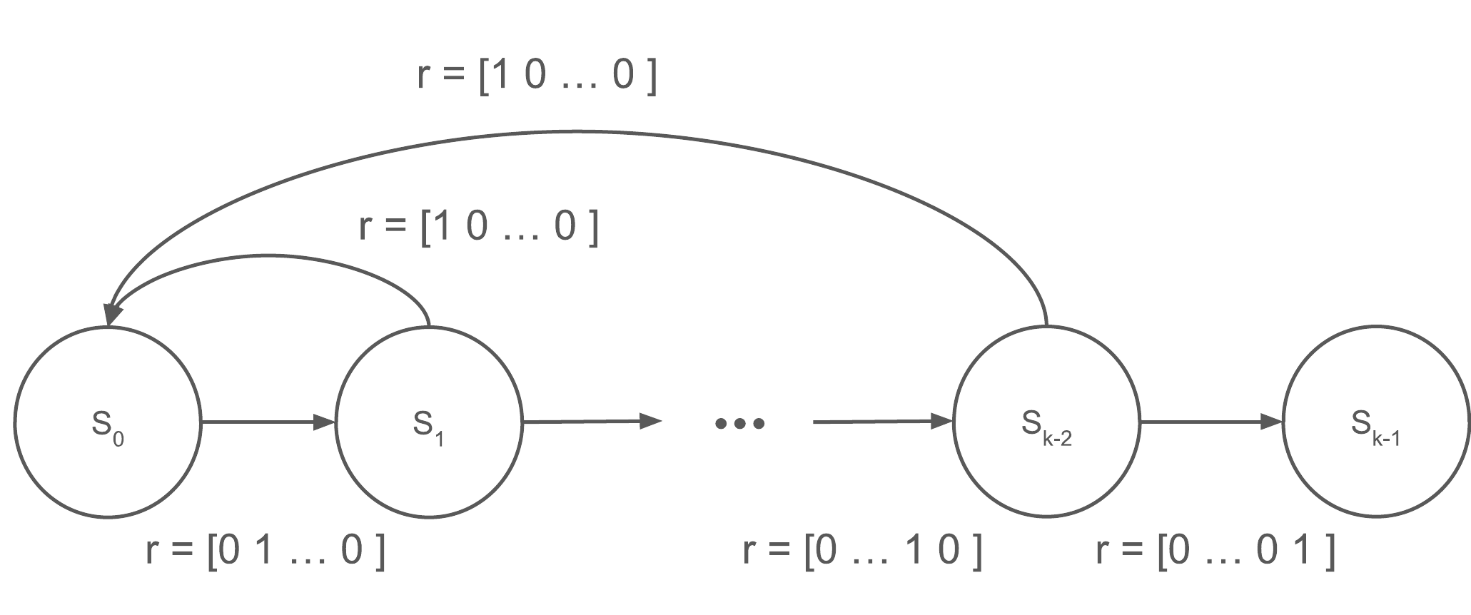
Chain environment.
The chain is a controlled policy-evaluation setup. Because the transition dynamics are tabular and simple, it lets us compare two Bellman-target constructions directly.
In standard one-sample TD, each update observes one transition and bootstraps from the single sampled successor. For a transition from state $s_i$, this means the target particles come from whichever successor was sampled on that update. This is the usual stochastic TD regime.
The chain also lets us build a near-exact version of true distributional TD. Instead of using only the sampled successor, we explicitly construct the transition-mixture target: with probability $0.9$ the forward action moves to $s_{i+1}$, and with probability $0.1$ it resets to $s_0$. We back up both successor distributions and resample particles from that mixture. This approximates the population distributional Bellman target much more closely while keeping the same finite particle budget.
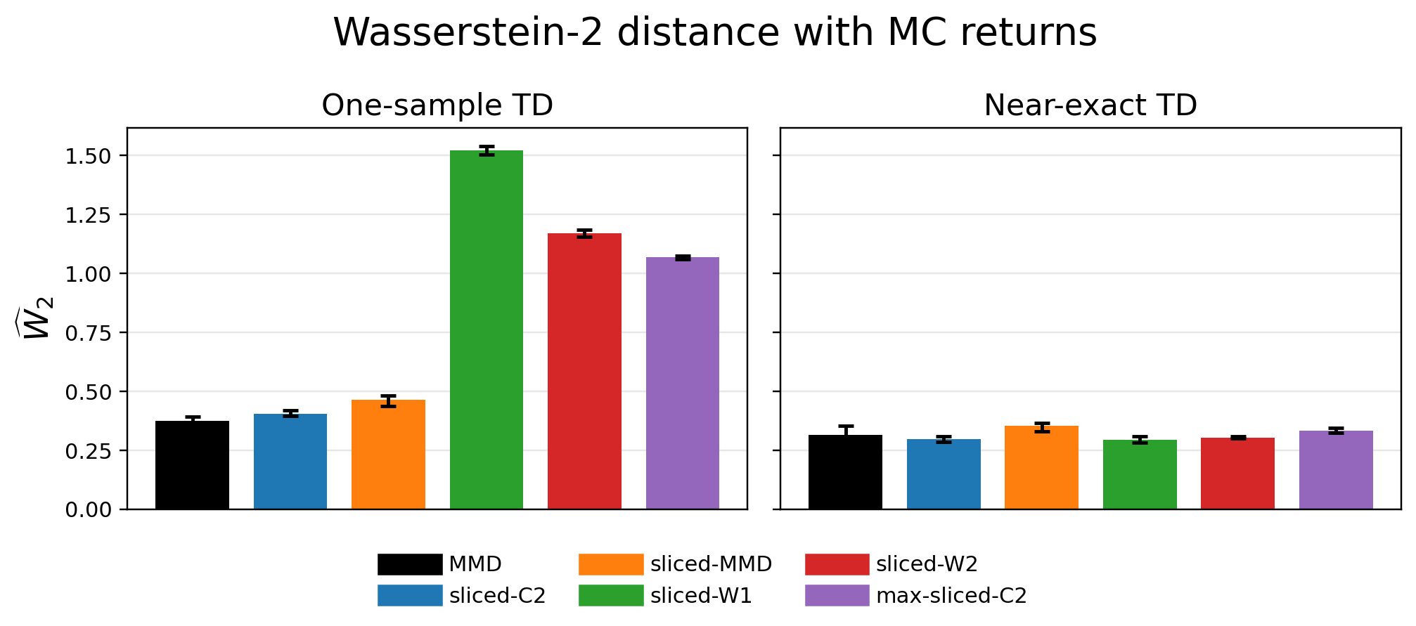
The bar plot reports empirical $\widehat{\mathbf W}_2$ between Monte Carlo returns and the critic's learned particle distribution at the start state. Lower is better: it means the learned return law is closer to the rollout distribution. Under near-exact distributional TD, the bias from the sampled target largely disappears. Under ordinary one-sample TD, objectives that violate the unbiased sample-gradient property degrade sharply.
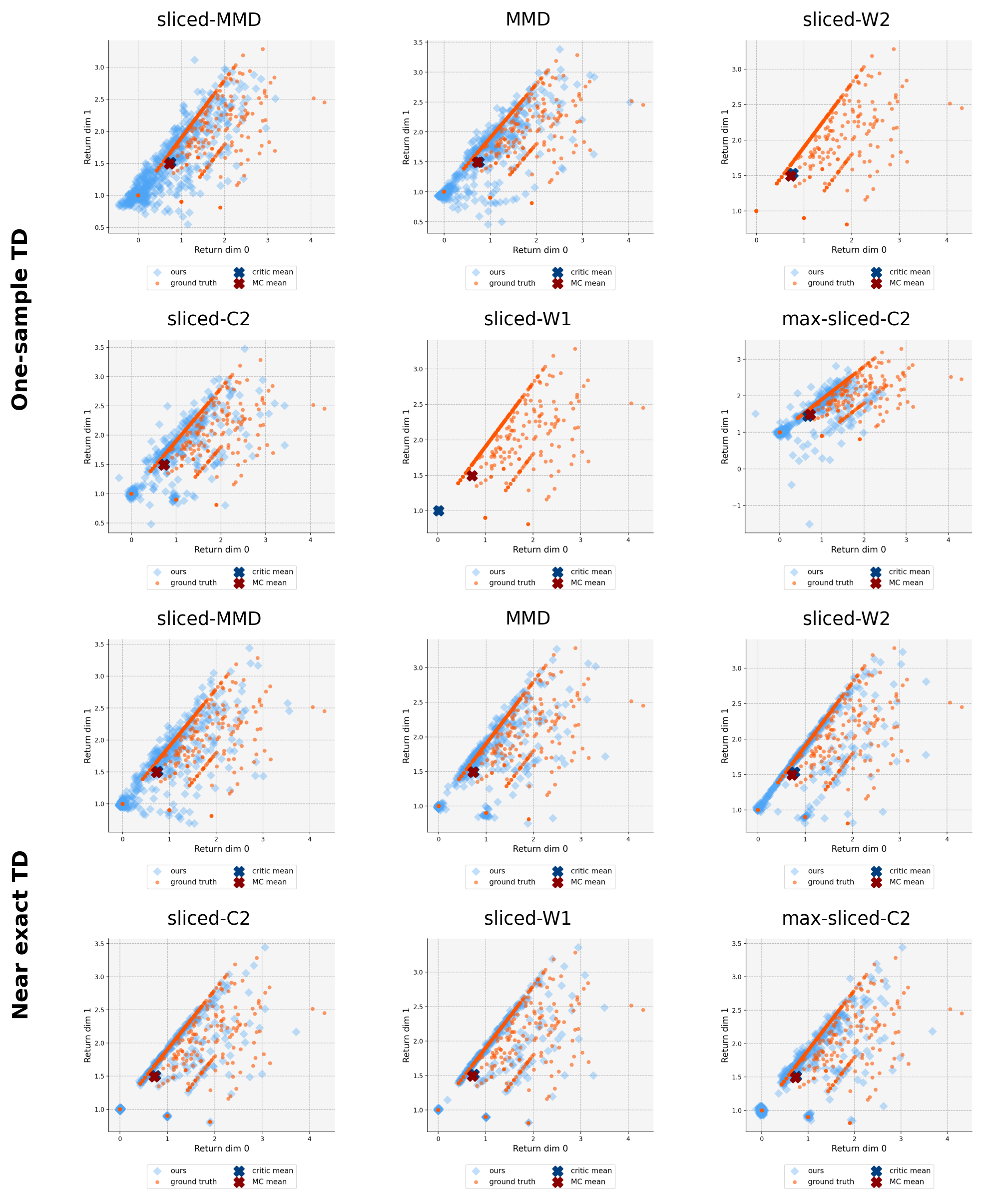
Figure 11 shows the same point directly in return space. Orange points are Monte Carlo rollout returns; blue diamonds are critic particles. The red and blue crosses mark the corresponding means. The near-exact update gives a much cleaner distributional match, while one-sample TD exposes the collapse or mismatch of objectives that are not compatible with the sampled target.
Maze from pixels.
The maze experiments are also policy evaluation, but now from pixel observations and vector-valued rewards, following the multi-dimensional reward setting of Zhang et al. [5]. Unlike the tabular chain, the exact transition-mixture target is not constructed here; training uses the usual sampled TD target. So the maze reuses the same issue introduced by the chain, but in a pixel-based setting.
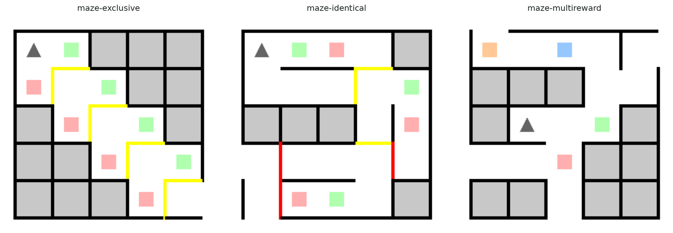
The agent receives an $84\times84\times3$ RGB rendering of the maze. In the three examples below, the grey triangle is the agent, grey blocks and black walls are obstacles, and colored squares are reward sources. The reward is vector-valued: reaching a colored square emits a stochastic reward in the corresponding component, and that source cannot be collected again in the same episode. Colored wall segments add one-way movement constraints: yellow walls can be crossed from the top or from the left, while red walls can be crossed from the bottom or from the right. So the critic has to infer from pixels which reward components are reachable, and how the resulting return coordinates vary together over a rollout.
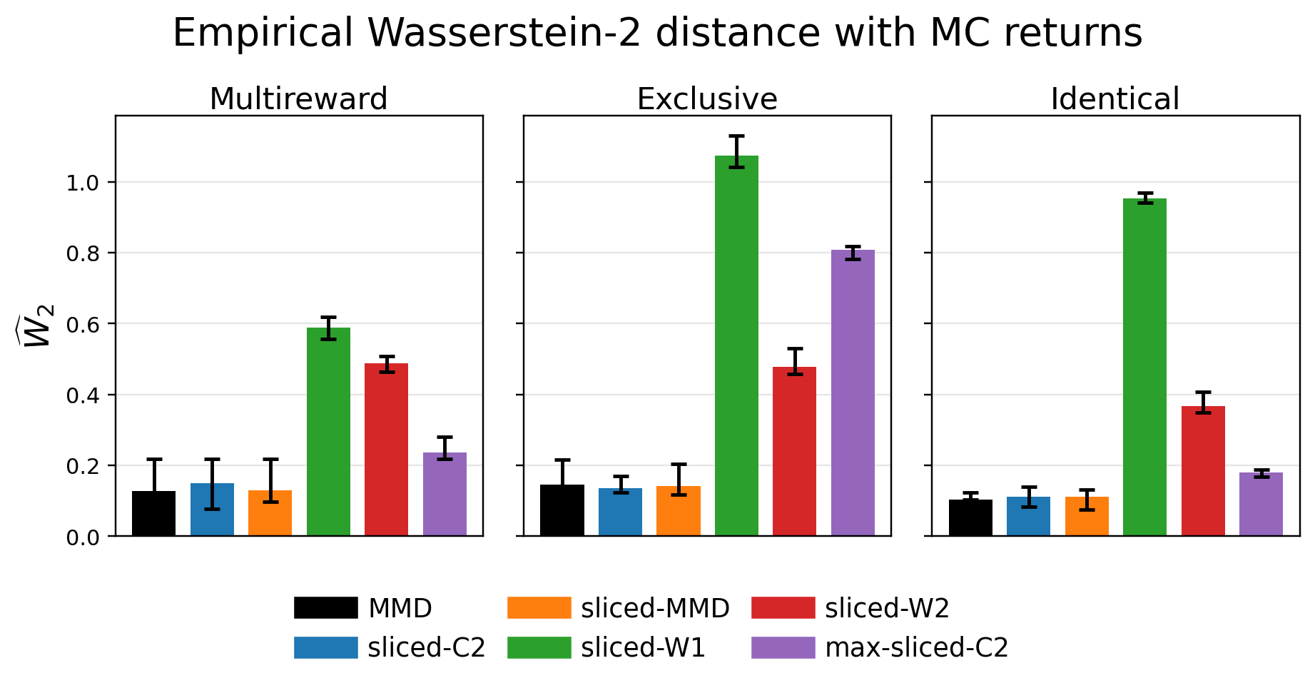
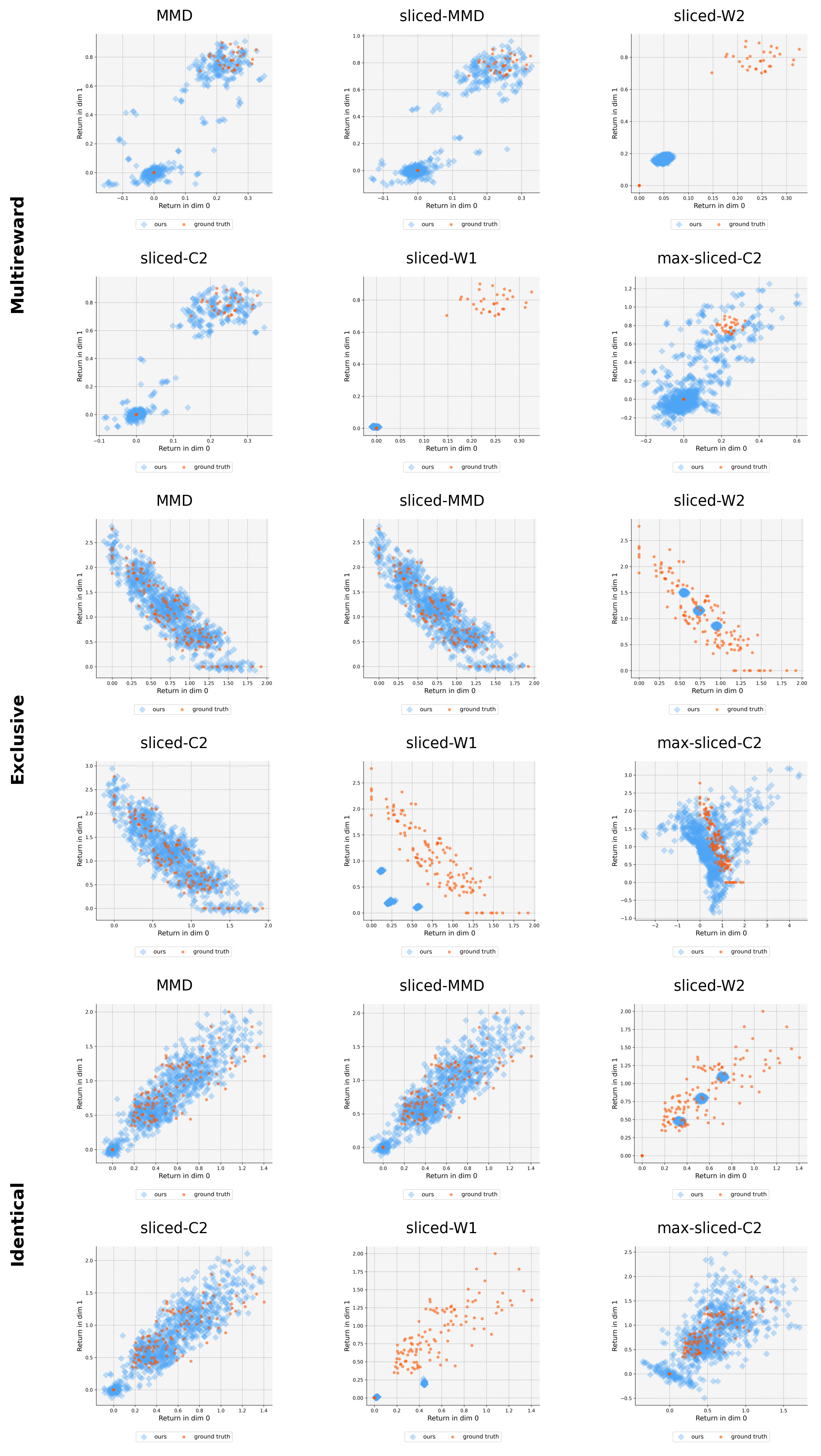
The maze bar plot again reports empirical $\widehat{\mathbf W}_2$ between Monte Carlo returns and critic particles, now across the three maze variants. Figure 12 gives the corresponding particle-cloud view: orange points are rollout returns and blue diamonds are critic particles. The rows are the maze variants, and the columns are the distributional objectives. The important visual check is whether the learned particles cover the same cloud as the rollout returns, not only whether their average is in the right area.
Atari control.
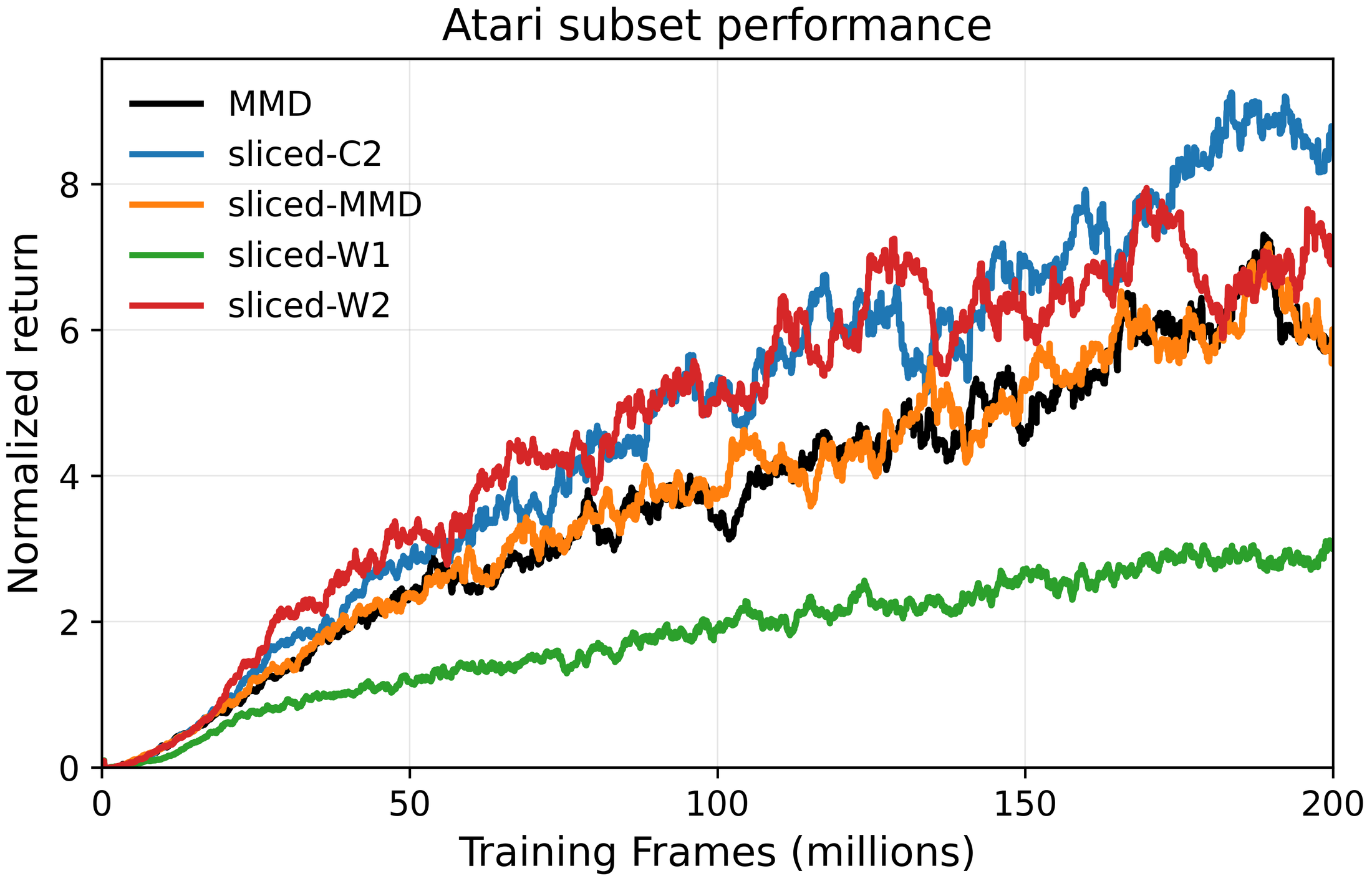
The Atari subset tells a slightly different story, again using decomposed reward signals [5]. Sliced Cramér performs strongly, but sliced Wasserstein can also work very well for control despite looking worse as a distributional matching objective in earlier experiments.
That is not a contradiction. Policy improvement depends heavily on expected return estimates. An objective can model the full return distribution poorly and still give useful expectations for control. For policy evaluation, that is not enough; for control, it may sometimes be enough.
Practical takeaway
For multivariate distributional policy evaluation with standard one-sample TD, sliced Cramér is the safest default.
Sliced MMD is mainly a kernel-based comparison point. It gives freedom to choose the kernel, but in this setting it does not bring a clear advantage over sliced Cramér and it keeps the usual quadratic cost in the number of particles.
Sliced Wasserstein is not appropriate as a distributional learning objective under one-sample stochastic TD. Its Atari control performance should not be read as evidence that it learns the return distribution well: the experiments show that it can still produce a control-useful signal while collapsing the distributional information that policy evaluation is meant to preserve.
Max slicing is theoretically valuable for matrix-discounted Bellman operators [10], but its sample-dependent direction selection makes it inappropriate for one-sample stochastic TD [2] [4].
Open question
The clean open question is whether we can get all of the following at once:
- norm-only contraction under general matrix discounts,
- compatibility with one-sample TD,
- tractable estimators,
- dimension-friendly statistical rates.
In paper notation, the dream is a divergence $\mathcal D$ such that
$$ \overline{\mathcal D}(\mathcal T^\pi\eta_1,\mathcal T^\pi\eta_2) \le c(\bar L)\,\overline{\mathcal D}(\eta_1,\eta_2), \qquad \bar L = \sup_{s,a}\|\Gamma(s,a)\|_{\mathrm{op}}, $$
while still behaving correctly when the Bellman target is sampled through the usual one-sample TD update.
We left this as an open question.
Bibliography
- Bellemare, Dabney, and Munos, 2017. A Distributional Perspective on Reinforcement Learning. arXiv.
- Bellemare, Danihelka, Dabney, Mohamed, Lakshminarayanan, Hoyer, and Munos, 2017. The Cramér Distance as a Solution to Biased Wasserstein Gradients. arXiv.
- Dabney, Rowland, Bellemare, and Munos, 2018. Distributional Reinforcement Learning with Quantile Regression. arXiv.
- Rowland, Dadashi, Kumar, Munos, Bellemare, and Dabney, 2019. Statistics and Samples in Distributional Reinforcement Learning. arXiv.
- Zhang, Chen, Zhao, Xiong, Qin, and Liu, 2021. Distributional Reinforcement Learning for Multi-Dimensional Reward Functions. OpenReview.
- Wiltzer, Farebrother, Gretton, and Rowland, 2024. Foundations of Multivariate Distributional Reinforcement Learning. arXiv.
- Rabin, Peyré, Delon, and Bernot, 2011. Wasserstein Barycenter and its Application to Texture Mixing. Springer.
- Bonneel, Rabin, Peyré, and Pfister, 2015. Sliced and Radon Wasserstein Barycenters of Measures. Springer.
- Nadjahi, Durmus, Chizat, Kolouri, Shahrampour, and Simsekli, 2020. Statistical and Topological Properties of Sliced Probability Divergences. arXiv.
- Deshpande et al., 2019. Max-Sliced Wasserstein Distance and Its Use for GANs. arXiv.
- Gretton, Borgwardt, Rasch, Schölkopf, and Smola, 2012. A Kernel Two-Sample Test. JMLR.
- Nguyen-Tang, Gupta, and Venkatesh, 2021. Distributional Reinforcement Learning via Moment Matching. arXiv.
- Killingberg and Langseth, 2023. The Multiquadric Kernel for Moment-Matching Distributional Reinforcement Learning. OpenReview.
- Barreto et al., 2017. Successor Features for Transfer in Reinforcement Learning. arXiv.
- Debes and Tuytelaars, 2026. Distributional Value Gradients for Stochastic Environments. arXiv.
- Hessel, Modayil, van Hasselt, Schaul, Ostrovski, Dabney, Horgan, Piot, Azar, and Silver, 2018. Rainbow: Combining Improvements in Deep Reinforcement Learning. arXiv.
- Felten, Alegre, Nowé, Bazzan, Talbi, Danoy, and da Silva, 2023. A Toolkit for Reliable Benchmarking and Research in Multi-Objective Reinforcement Learning. Proceedings of NeurIPS 2023. OpenReview.
- Fedus, Gelada, Bengio, Bellemare, and Larochelle, 2019. Hyperbolic Discounting and Learning Over Multiple Horizons. arXiv.