When Is Distributional RL with MMD Well Founded ?
It is well founded when the distributional Bellman operator is a contraction in MMD. We reduce this to a criterion on the kernel and use it to find new kernels that induce contraction. Surprisingly, we show that kernels that induce faster contraction tend to be less able to tell distributions apart.
Distributional reinforcement learning predicts the whole distribution of returns, not only their mean [1]. One needs to compare the predicted distribution with a target one. One way to compare them is a kernel distance called the Maximum Mean Discrepancy (MMD) [2] [3]. MMD is attractive because it is reasonably fast to estimate and only needs samples.
The target is given by the distributional Bellman operator. It adds the reward of the current step to the discounted return predicted at the next state. The prediction is moved toward the target by minimizing the MMD between them. For this to be well founded, the Bellman operator must be a contraction in MMD: applying it to any two predictions reduces the MMD between them by at least a fixed factor. Repeated updates then converge to the true return distribution.
Whether the Bellman operator is a contraction in MMD depends on the kernel. Some results were known, but they covered only a few kernels and could not be extended to find others [3] [4] [5]. Our work makes five contributions.
- A kernel test. Checking contraction reduces to testing a property of a kernel built from the original one.
- Radial kernels. For radial kernels, we use Schoenberg's theorem and Bernstein functions to turn this test into a criterion on the radial profile of the kernel. It confirms already known results and reveals when contraction is impossible. Using it in a numerical search, we find 11 new kernel families that induce contraction.
- The RBF puzzle. The RBF kernel does not induce contraction in general but performs very well in practice. This seems to be a contradiction. Our numerical tests give a partial explanation: they suggest that the RBF kernel induces contraction when returns stay in a range that is small compared with its lengthscale.
- Chaining. A carefully tuned sum of RBF kernels gives a kernel that induces contraction with a chosen factor.
- A tradeoff. There is a tradeoff between contraction and the ability to tell distributions apart from limited data. Faster contraction should therefore not necessarily be the target.
Table of contents
- Distributional RL and MMD
- Why contraction matters
- From contraction to a kernel test
- Radial kernels and Bernstein functions
- The RBF puzzle
- Chaining RBF kernels
- Faster is not always better
- Open questions
- Bibliography
Distributional RL and MMD
We consider a Markov decision process with discount factor $\gamma$ and a fixed policy $\pi$. Starting from a state $s$ and an action $a$, the return $Z^\pi(s,a)$ is the discounted sum of future rewards. It is a random variable whose mean is the Q-value $Q^\pi(s,a)$:
Distributional RL learns the whole distribution $\eta^\pi(s,a)$ of the return instead of only its mean.
Given a prediction $\eta$, the distributional Bellman operator $\mathcal T^\pi$ gives the distribution of the reward plus the discounted return predicted at the next state:
Here $P(\cdot\mid s,a)$ is the distribution of the next state $S'$, the next action $A'$ is drawn from the policy, and $X'$ from the prediction at $(S',A')$. The true return distribution is a fixed point of this operator: $\eta^\pi=\mathcal T^\pi\eta^\pi$.
A common choice is to represent each predicted distribution $\eta(s,a)$ by equally weighted particles [3].
MMD compares a prediction with its target through a kernel: a symmetric function $k(x,y)$ that scores how similar two returns are. The squared MMD between two distributions $\mu$ and $\nu$ is
The choice of kernel controls which aspects of the distributions are compared and how sensitively. For example, the kernel $k(x,y)=-\|x-y\|^2$ gives
so MMD cannot tell apart two distributions with the same mean.
When both distributions are given by particles $x_1,\dots,x_n$ and $y_1,\dots,y_m$, the expectations become averages over all pairs of particles:
Returns can also be vectors in $\mathbb R^d$, for example when the reward has several components [6] [7] [8]. MMD applies without change, and the contraction results of the paper hold in any dimension.
Why contraction matters
A prediction $\eta$ gives one distribution for each state and action. To compare two predictions $\eta_1$ and $\eta_2$, we take the largest MMD over all states and actions:
This is the supremum MMD [1] [3]. Two predictions are close in this sense only if they are close at every state and action.
We say that $\mathcal T^\pi$ is a contraction with factor $\tau\in[0,1)$ if it shrinks the squared supremum MMD between any two predictions $\eta_1$ and $\eta_2$ by at least that factor:
Any such $\tau$ is a contraction factor. We write $\tau^\star_k$ for the smallest factor that holds for every MDP with discount $\gamma$ and every policy. All factors in this post refer to the squared supremum MMD, and the factor for the supremum MMD itself is the square root.
When $\tau^\star_k<1$, the equation $\eta^\pi=\mathcal T^\pi\eta^\pi$ has a unique solution. Applying $\mathcal T^\pi$ $n$ times to any prediction $\eta$ then gives
The smaller the factor, the faster this bound goes to zero.
Before this work, contraction had been settled for three kernels. Table 1 summarizes these results [3] [4] [5].
| Kernel | Formula | Contraction in squared supremum MMD |
|---|---|---|
| Power-distance [3] | $k_\alpha(x,y)={}$$-\|x-y\|^\alpha$ $0<\alpha\le 2$ | Yes, factor $\gamma^\alpha$ |
| Gaussian RBF [3] | $k(x,y)={}$$\exp\!\big(-\|x-y\|^2/\ell^2\big)$ | No in general |
| Multiquadric [4] [5] | $k(x,y)={}$$-\sqrt{1+\|x-y\|^2/\ell^2}$ | Yes, factor $\gamma$ |
For returns in $\mathbb R^d$, Wiltzer et al. proved contraction in MMD only for a narrow class of kernels that includes the power-distance kernels [7].
From contraction to a kernel test
Our first result turns contraction into a property of a kernel, which needs one definition. A symmetric kernel $k$ is conditionally positive definite (CPD) when every choice of points $x_1,\dots,x_n$ and of weights $w_1,\dots,w_n$ summing to zero gives
Interestingly, if a kernel $k$ is CPD, the squared MMD built from it is never negative (the converse also holds).
The result needs one more definition. For a factor $\tau\in[0,1)$ and a reward value $q$, we define the Bellman difference kernel of $k$ as
With this kernel, we can state our first main result.
In other words, checking contraction no longer requires looking at MDPs at all: it is enough to check that the Bellman difference kernel is CPD for every reward value.
This also works the other way round. When the test fails, some MDP with discount $\gamma$ and some policy break contraction with factor $\tau$.
Radial kernels and Bernstein functions
The kernels used with MMD in distributional RL, such as the RBF and multiquadric kernels, only depend on how far apart two returns are. Kernels of this kind are called radial: they can be written $k(x,y)=g(\|x-y\|)$ for a function $g$ of the distance. The function $g$ is the kernel's radial profile.
Radial kernels have a nice property: their Bellman difference kernel simplifies to
The reward value $q$ of the original definition is gone. For radial kernels, contraction depends only on the radial profile $g$ and the discount $\gamma$.
The question becomes: when is a radial kernel CPD ? Schoenberg's theorem answered this question in 1938 [9].
A radial kernel is CPD in every dimension
exactly when $\phi(r^2):=g(0)-g(r)$ is a Bernstein function.
A Bernstein function is a function $\phi$ on $[0,\infty)$ of the form below, with $b\ge 0$ and $\Lambda$ a positive measure on $(0,\infty)$:
We call $b$ the drift and $\Lambda$ the Lévy measure of $\phi$. The Lévy measure says how much each term $1-e^{-st}$ contributes. As we will see, these two decide whether a kernel induces contraction.
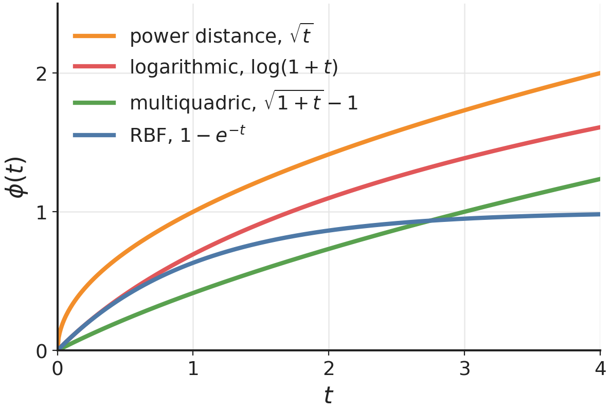
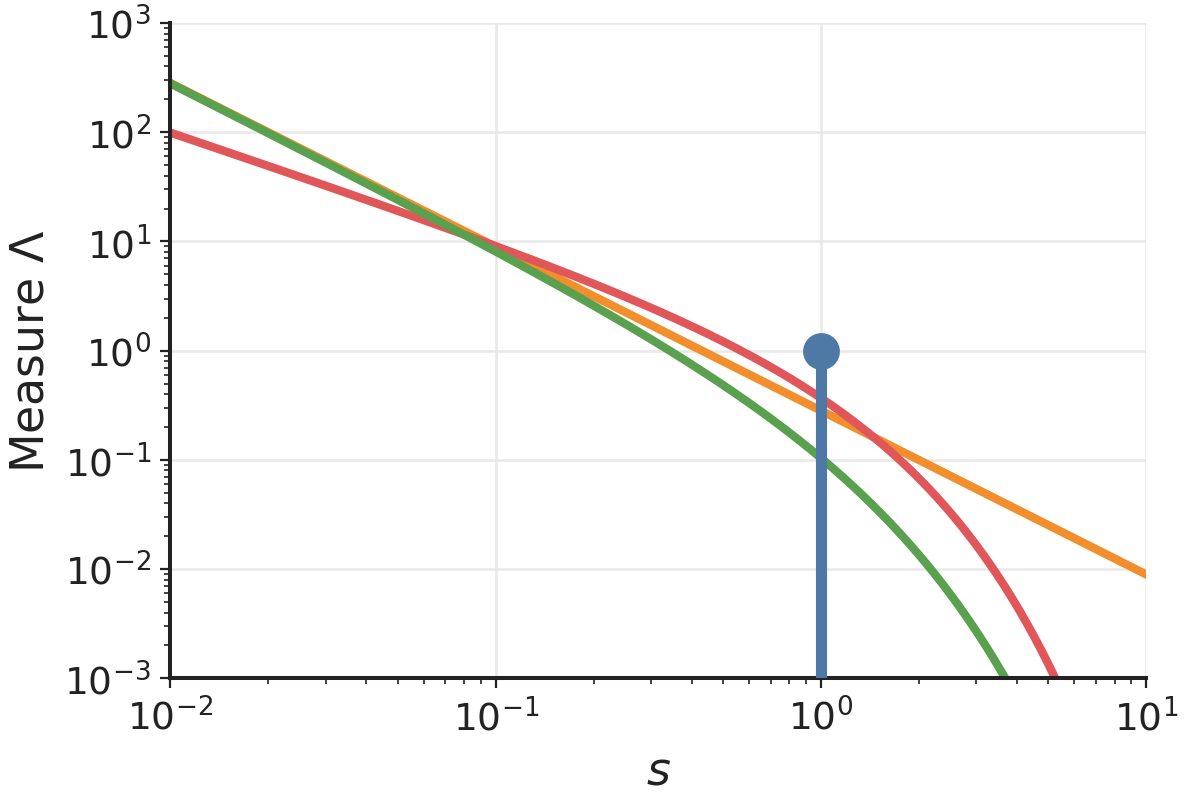
Figure 1. Examples of Bernstein functions (left) and their Lévy measures (right). The RBF measure is a single atom. The others are continuous.
Figure 1 shows four examples. The RBF profile $1-e^{-t}$ saturates at 1. The other three keep growing. Why does only the RBF profile saturate ? The right panel shows it. The RBF profile is a single term $1-e^{-t}$. Its measure is one point that carries all the weight. Such a point is called an atom. The other three add up terms $1-e^{-st}$ with smaller and smaller $s$. These terms saturate later and later. Their sum keeps growing.
As we saw, the Bellman difference kernel of a radial kernel is itself radial. Schoenberg's theorem therefore applies to it, with the function
This leads to our second main result.
Here is the interesting part: whether $\psi_\tau$ is a Bernstein function can be read directly from the drift $b$ and the Lévy measure $\Lambda$ of $\phi$. It is one exactly when
The set $B/\gamma^2=\{s/\gamma^2 : s\in B\}$ is obtained by dividing every point of $B$ by $\gamma^2$. Since $\gamma<1$, dividing by $\gamma^2$ makes every point larger. In words, the weight that $\Lambda$ puts near any value $s$ must be matched by at least $1/\tau$ times as much weight near the smaller value $\gamma^2 s$.
So does the criterion agree with what we already know ? It recovers all the known results. It gives the factor $\gamma^\alpha$ for the power-distance kernels and $\gamma$ for the multiquadric kernel. It also explains why the RBF kernel fails, as we show.
When contraction is impossible
The criterion also reveals when contraction is impossible. A first obstruction comes from profiles that saturate. Remember the RBF profile saturating in Figure 1 ? This is exactly what rules it out. A kernel whose profile saturates never induces contraction.
A second obstruction comes from the Lévy measure. If $\Lambda$ has at least one atom but only finitely many, contraction fails in some dimension. This rules out the RBF kernel again because its $\Lambda$ is a single atom. It also rules out every finite sum of RBF kernels.
Searching for new kernels
The criterion also lets us look for new kernels. It takes a simple form for a special case called complete Bernstein functions. For them, checking the criterion comes down to finding the maximum of a function of one variable. A reference book lists many Bernstein functions with the density of their Lévy measure [10]. We compute this maximum numerically for 43 of them. The search finds 11 new kernel families that induce contraction. Table 2 shows three of them next to the two kernels known before.
| Kernel $k(x,y)$ | Contraction | Shown |
|---|---|---|
| $-r^\alpha$ | $0<\alpha\le 2$, factor $\gamma^\alpha$ | proved [3] |
| $-\big(1+r^2/\ell^2\big)^\beta$ | $0<\beta\le 1$, factor $\gamma^{2\beta}$ | proved, $\beta=1/2$ in [4] [5] |
| $-\dfrac{r^2}{(r^2+\ell^2)^\alpha}$ | $0<\alpha\le 3/4$ | numerically, new |
| $-r\,\big(1-e^{-r/\ell}\big)$ | every $\ell$ | numerically, new |
| $-r\arctan(r/\ell)$ | every $\ell$ | numerically, new |
The RBF puzzle
The RBF kernel is one of the most common kernels for MMD in distributional RL. It also performs among the best in practice [3]. Yet we saw that it does not induce contraction. How can both be true ?
Part of the answer comes from a property of many RL problems: rewards are bounded. If every reward has norm at most $r_{\max}$, every return lies in the ball of radius $r_{\max}/(1-\gamma)$. A Bellman update also keeps predictions inside this ball.
This changes the question. Contraction no longer needs the Bellman difference kernel to be CPD everywhere. It only needs it on the ball.
We test this numerically on random sets of points drawn in the ball. On each set, we compute the smallest factor that passes the test. A test on finitely many points can rule contraction out. It cannot prove it.
Figure 2 shows the result in one dimension. The RBF kernel passes the test when the ball is small compared with its lengthscale. In the hatched region it fails, and contraction on the ball is impossible. The logarithmic kernel also fails to induce contraction in general. On the ball, it passes the test at every radius shown. This may explain part of the RBF kernel's success. Proving contraction on the whole ball remains open.
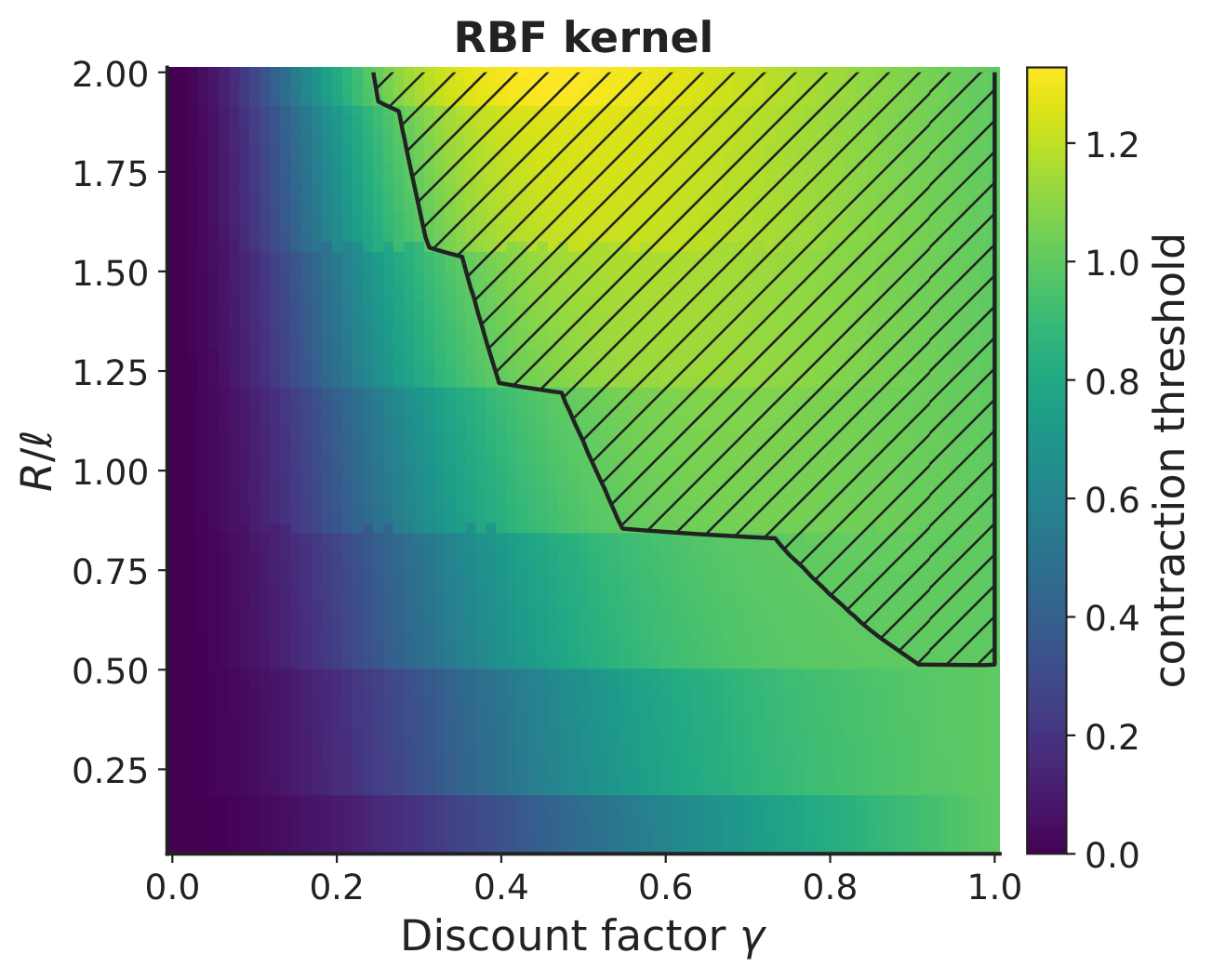
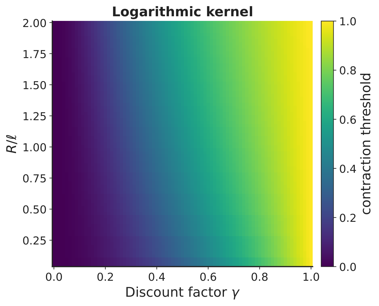
Figure 2. Largest factor found on random sets of points in a ball of radius $R$, for the RBF kernel (left) and the logarithmic kernel (right). In the hatched region it exceeds 1.
Chaining RBF kernels
Can RBF kernels induce contraction at all ? A single one cannot, and neither can a finite sum. Surprisingly, a carefully chosen infinite sum can. We call this construction chaining.
Write $k_\ell(x,y)=\exp(-\|x-y\|^2/\ell^2)$ for the RBF kernel with lengthscale $\ell$. Given a target factor $\tau$, the chained RBF kernel is
From one term to the next, the lengthscale grows by a factor $1/\gamma$ and the weight by a factor $1/\tau$. Each new term is sensitive to larger distances between returns and counts more.
This kernel gives our third main result.
Figure 3 shows the profile of the chained RBF kernel for three target factors. Each RBF term saturates. Their sum keeps growing. The smaller $\tau$, the faster it grows. Remember the second obstruction ? Finitely many atoms in the Lévy measure rule out contraction. On the right, each RBF term of the chain is one atom. The chain has infinitely many of them.
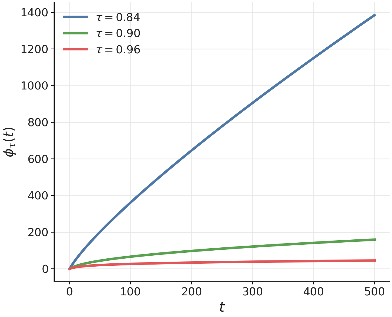
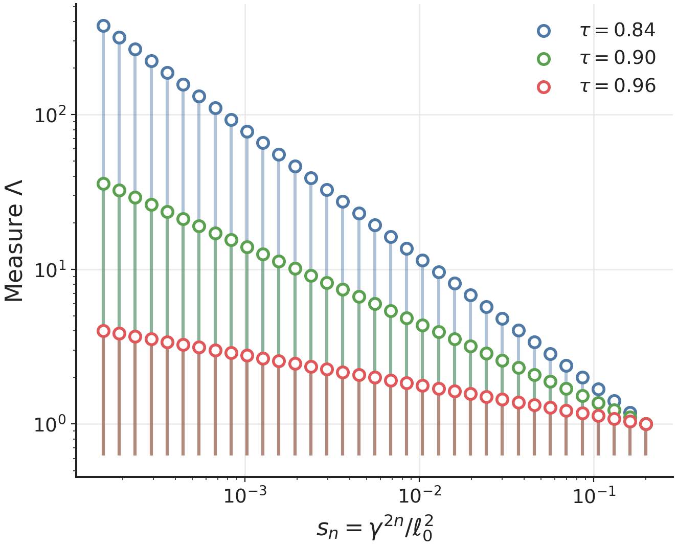
Figure 3. Profile (left) and Lévy measure (right) of the chained RBF kernel for three target factors $\tau$, with $\gamma=0.9$.
We know of no closed form for the chained kernel. To compute it, we truncate the sum and keep only its first terms. The result is a finite sum of RBF kernels. As we saw, contraction then fails in some dimension. The test on a ball from the previous section still applies. In our tests, about a dozen terms are enough to pass it. With more terms, the factor found on the ball gets closer to that of the full chain.
Chaining gives a new kernel for distributional RL with MMD. We can choose its contraction factor. But is a smaller factor always better ?
Faster is not always better
Not necessarily. Changing the kernel changes more than the contraction factor. It also changes which differences between two distributions the MMD can detect. A kernel that contracts faster may detect less.
Remember the kernel $-\|x-y\|^2$ from the first section ? Its MMD only compares means. Interestingly, it is the only kernel that reaches the smallest possible factor $\gamma^2$. Every other kernel built from a Bernstein function can tell any two distributions apart. Its factor is always above $\gamma^2$.
How can we measure what a kernel detects ? MMD is also a classic statistical test [2]. Given samples from two distributions, it decides whether they differ. The power of the test is how often it detects a difference that is really there.
Figure 4 shows one such test. The two samples on the left form a checkerboard. The test shuffles their labels many times. This shows how large the MMD gets when both samples come from the same distribution. The MMD of the actual samples is far larger. The test detects the difference.
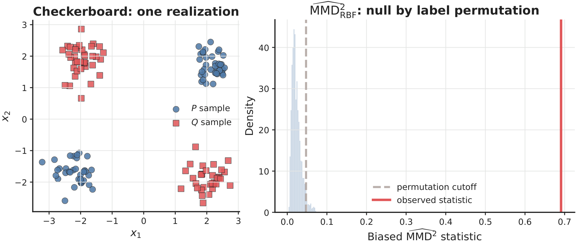
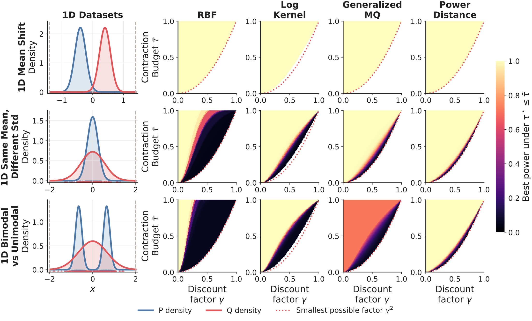
We run this test for four kernel families: RBF, logarithmic, generalized multiquadric and power distance. Each family has a parameter, such as the RBF lengthscale. For each discount $\gamma$ and each limit on the factor, we keep the family's most powerful kernel whose factor stays under the limit. The factor is computed on a ball that contains the data, as in the RBF puzzle.
Figure 5 shows the result in one dimension. The color is the best power under each limit on the factor. Bright colors mean high power. When the two distributions differ only in their mean, every kernel keeps its power. When they have the same mean but different spreads, or one peak against two, the power drops as the limit approaches $\gamma^2$. For the RBF kernel, it drops long before.
In the paper's appendix, the pattern holds up to 64 dimensions.
Faster contraction should therefore not be the only target. The right kernel depends on which differences between distributions matter for the task.
Open questions
We still do not know which kernels work best in practice, found or not yet found. The next step is to compare them on control tasks in RL environments, including the new ones.
How strong is the tradeoff in a real task ? It depends on the two distributions being compared. In distributional RL, these are the predicted and target returns. Measuring the tradeoff on the returns that arise during training could guide the choice of kernel.
Finally, can we prove that the RBF kernel induces contraction when returns stay in a range that is small compared with its lengthscale ? Our numerical tests suggest so. A proof is still open.
Bibliography
- Bellemare, Dabney, and Munos, 2017. A Distributional Perspective on Reinforcement Learning. arXiv.
- Gretton, Borgwardt, Rasch, Schölkopf, and Smola, 2012. A Kernel Two-Sample Test. JMLR.
- Nguyen-Tang, Gupta, and Venkatesh, 2021. Distributional Reinforcement Learning via Moment Matching. arXiv.
- Killingberg and Langseth, 2023. The Multiquadric Kernel for Moment-Matching Distributional Reinforcement Learning. OpenReview.
- Debes and Tuytelaars, 2026. Distributional Value Gradients for Stochastic Environments. arXiv.
- Zhang, Chen, Zhao, Xiong, Qin, and Liu, 2021. Distributional Reinforcement Learning for Multi-Dimensional Reward Functions. OpenReview.
- Wiltzer, Farebrother, Gretton, and Rowland, 2024. Foundations of Multivariate Distributional Reinforcement Learning. arXiv.
- Debes and Tuytelaars, 2026. Multivariate Distributional Reinforcement Learning Using Sliced Divergences. arXiv.
- Schoenberg, 1938. Metric Spaces and Positive Definite Functions. Transactions of the AMS.
- Schilling, Song, and Vondraček, 2009. Bernstein Functions: Theory and Applications. De Gruyter.