Slicing Return Distributions: A Practical Route to Multivariate Distributional RL
How can we learn the joint distribution of several returns ? We compare return distributions through their one-dimensional projections. This makes the comparison cheap. Only some of these sliced divergences keep the unbiased gradients that TD learning needs.
Distributional RL models the distribution over returns instead of their expectation [1]. In the usual case of a single reward dimension, this is already useful. The mean alone does not show how much returns vary, whether their distribution is skewed, or whether it has several peaks. This also allows risk-aware action selection, for example by giving more weight to poor outcomes [19]. Distributional RL was also an important part of Rainbow's improvements over DQN [16].
What changes when the reward has several dimensions ? The return becomes a vector. Its joint distribution tells us how the components vary together [6]. Multi-objective RL is one example, with reward components that can compete [17]. Successor features [14] and value-gradient methods [15] are others. Both use temporal difference updates with targets that have several dimensions.
But comparing multivariate distributions can be much more expensive than comparing 1D distributions. In this work, we use a trick from optimal transport called slicing [7] [8] [9]. It compares high-dimensional distributions through their 1D projections along many directions. We combine slicing with TD learning to learn return distributions. As we discuss below, this leaves some questions open.
Table of contents
- Why multivariate distributional RL ?
- What makes the multivariate case difficult ?
- The slicing trick
- Which 1D divergence should we use slicing with ?
- From sliced divergences to a TD update
- Uniform slicing vs max slicing
- What the theory says
- Does one-sample TD give the right gradients ?
- Experiments
- Practical takeaway
- Open question
- Bibliography
Why multivariate distributional RL ?
For a fixed policy $\pi$, the usual scalar return is a discounted sum of rewards,
With several reward components, we would like to predict their joint return distribution. Learning each component separately would not tell us how they vary together. For example, two objectives might both have high returns on the same trajectories. Or improving one might lower the other.
We can write a multivariate return as
Here $R_t$ is a reward vector. The discount $\Gamma(s,a)$ can be $\gamma I_d$. This applies the same discount to every component. A more general matrix can apply different discounts or mix the components.
The corresponding distributional Bellman update is
As in scalar RL, we combine the immediate reward with a discounted prediction at the next state. The difference is that the prediction is now a joint distribution over several return components.
What makes the multivariate case difficult ?
Why not just add more outputs to the usual 1D distributional critic ? Each distributional RL method combines two choices : 1) how to represent the distribution and 2) how to compare distributions. Neither choice extends easily from 1D to several dimensions.
C51 models the distribution over returns by placing probabilities on a fixed grid [1]. Extending that grid to $d$ dimensions would require $m^d$ grid points for $m$ values per dimension. Quantile methods instead rely on ordering the returns [3]. Scalar samples can be sorted from smallest to largest, but multivariate samples have no obvious equivalent ordering.
What about simply using the Wasserstein distance ? In 1D, its empirical estimator is cheap to compute because it relies on sorting. In several dimensions, solving the optimal transport problem is much more expensive [6]. With $n$ samples, the costs can differ substantially.
| Problem | Typical empirical cost |
|---|---|
| 1D Wasserstein by sorting | $\mathcal O(n \log n)$ |
| exact multivariate OT | often around $\mathcal O(n^3 \log n)$ |
We would pay that cost at every TD update. Cost is not the only problem. The Wasserstein distance also suffers from the curse of dimensionality. In general, maintaining the same estimation accuracy can require exponentially more samples as the dimension increases [20].
The slicing trick
The slicing trick is simple. Instead of comparing the multivariate distributions directly, we look at them from many directions. Each time, we project them onto a line [7] [8] [9]. The figure below shows two projections of the same pair of distributions.
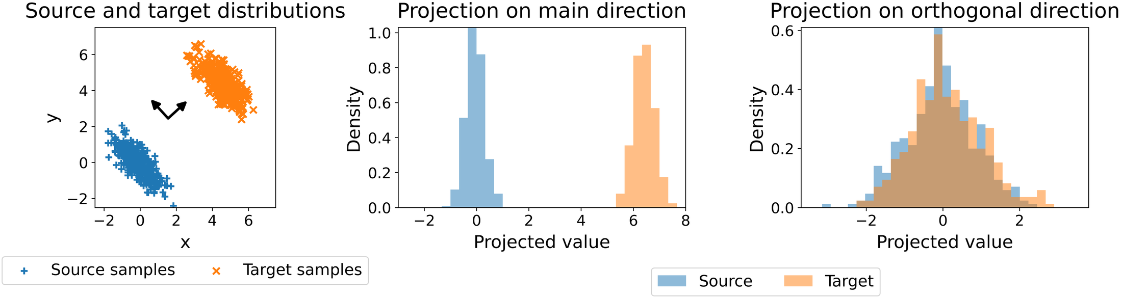
Choose a unit direction,
and project each vector $x \in \mathbb R^d$ onto it,
For distributions $\mu$ and $\nu$, the notation $(P_\theta)_\#\mu$ and $(P_\theta)_\#\nu$ means their distributions after projection. Both are in 1D. We can therefore compare them with a 1D divergence $\Delta$.
Uniform slicing averages these comparisons over all directions. We write the powered objective as
Here $\sigma$ is the uniform distribution over directions. In practice, we draw $L$ random directions and average their contributions,
With this estimator, we never compute a multivariate transport plan. We only compare 1D projections along many directions. Each of these 1D comparisons can be very cheap. The next section shows several ways to compare them.
Which 1D divergence should we use slicing with ?
Many divergences can be computed at a reasonable cost in 1D. Here we consider the Wasserstein distance, the Cramér distance and the Maximum Mean Discrepancy (MMD) [11]. To see how they are computed, suppose our prediction and target are each represented by $n$ particles,
Each particle is one possible return vector of the distribution we seek to model. For a direction $\theta$, simply project the particles,
Then we compute the 1D divergence between the two sets of projected particles. Finally, we average over the random directions.
Wasserstein. Let $u_i=P_\theta z_i$ and $v_i=P_\theta \hat z_i$ be the projected particles. Sort both bags and match the smallest values, then the next smallest, and so on. Writing the sorted values as $u_{(i)}$ and $v_{(i)}$, the empirical estimator is
Averaging over $L$ directions gives
Sorting costs $\mathcal O(n\log n)$ per projection. The loss is cheap to compute. But its gradient can be biased in TD learning [2] [4].
Cramér. This divergence compares cumulative distribution functions, or CDFs [2]. A CDF $F_\mu(t)$ gives the probability of a value at or below $t$. The Cramér distance integrates the squared difference between the two CDFs,
To compute it from particles, merge both bags of projected particles and sort again. Between consecutive values $t_k$ and $t_{k+1}$, the empirical CDF difference is constant. Calling that difference $\Delta_k$, we get
The sliced objective averages these values over directions,
Again, sorting is the main cost. Each projection takes $\mathcal O(n\log n)$. Unlike Wasserstein, the squared Cramér objective has the unbiased gradients needed for the stochastic TD updates considered here [2].
MMD. Maximum Mean Discrepancy uses a kernel $k$ to compare pairs of samples [11]. It is the only divergence considered here that remains practical to compute directly in several dimensions. It compares kernel values within each distribution with those between the two distributions,
With projected particles, the standard biased estimator is
Sliced MMD averages the kernel loss after projection [9],
Evaluating this estimator requires $\mathcal O(n^2)$ kernel evaluations per projection. This is the same cost as comparing the two sets of samples in their original space. The choice of kernel gives some freedom. Our later work studies which kernels can be used, with or without slicing [21]. Its blog post explains the results.
To summarize, the costs for one projection are
| Divergence | Time complexity |
|---|---|
| Wasserstein $\mathbf W_p$ | $\mathcal O(n\log n)$ |
| Cramér $\mathbf C_2$ | $\mathcal O(n\log n)$ |
| MMD$_k$ | $\mathcal O(n^2)$ |
MMD is also an existing baseline for distributional RL. Nguyen-Tang, Gupta and Venkatesh introduced it through moment matching [12]. Zhang et al. used it for multivariate rewards [5]. Wiltzer et al. studied its contraction for multivariate returns [6]. We compare against MMD on the full return vectors and against MMD after projection.
From sliced divergences to a TD update
How do we use these divergences as losses to train a critic ?
For each state-action pair $(s,a)$, the critic predicts $N$ return particles,
We sample an environment transition $(s,a,r,s')$ and a next action $a'\sim\pi(\cdot\mid s')$. Adding the reward to the discounted next-state particles gives the target,
We minimize a sliced divergence between the predicted and target particles. The target is treated as fixed. Here $\phi$ denotes the critic's parameters and $\phi^-$ the parameters used to construct the target.
This is the usual one-sample TD. The name refers to sampling one environment transition for the update, not to using just one critic particle. We can have many target particles. But they all come from the same sampled successor state and reward. They do not represent all the outcomes that could have followed $(s,a)$. To sample more of the possible transitions, we would need to rewind the environment to state $s$ and try action $a$ again. This is usually not possible.
Uniform slicing vs max slicing
So far, we have averaged over random directions. Another option is to search for the direction that best distinguishes the two distributions [10]. This gives max slicing,
In practice, we approximate the supremum by optimizing the direction on the unit sphere. This costs more than drawing random directions. But it can give a contraction guarantee that uniform slicing does not have. The difference appears when the discount is a general matrix rather than the same scalar for every return component.
What the theory says
With an exact Bellman update, we would like two different return predictions to move closer together. A contraction bound makes that precise. It tells us how much the distance between them shrinks after applying the operator.
Write $\eta(s,a)$ for a predicted return distribution. The operator is
The form of $\Gamma(s,a)$ determines which contraction results we can obtain.
Classical distributional RL. There is one return component and one discount factor,
Multivariate returns with a shared discount. Every component uses the same discount factor,
Suppose the base divergence satisfies the required translation, scaling and mixture conditions. Uniform slicing then gives
The overline takes the largest divergence across state-action pairs, and $c(\gamma)<1$ is the contraction factor.
Result 1. Uniform slicing preserves contraction with a shared scalar discount. For $\Gamma=\gamma I_d$, the sliced divergence inherits the contraction guarantee of its one-dimensional base divergence, under those conditions.
A fixed discount matrix. We can also use
For example, we might predict returns over different horizons by assigning a different discount factor to each component [18],
A discount matrix that depends on the state and action. More generally,
The off-diagonal entries allow one return component to contribute to the update of another. To bound the effect of these matrices, define
The operator norm measures the largest factor by which a matrix can stretch a vector. The contraction bound we would like to obtain depends only on $\bar L$,
We want $c(\bar L)<1$ whenever $\bar L<1$.
Result 2. Uniform slicing need not satisfy this bound for general discount matrices. Even when $\bar L<1$, we cannot generally bound its contraction using $\bar L$ alone. Some MMD constructions fail this bound as well.
The failure concerns this particular bound, not every possible contraction result.
Max slicing instead takes the most discriminative direction.
Result 3. Max slicing recovers the desired bound. Under the assumptions on the base divergence, it gives a contraction factor controlled by $\bar L$ for general discount matrices.
These results concern the Bellman operator applied to whole distributions. Our algorithm only sees samples. We still need to check what happens to its gradients.
Does one-sample TD give the right gradients ?
An essential property for stochastic TD is that the gradient from a sampled target agrees, on average, with the gradient for the full target. A contraction guarantee alone does not establish this [2] [4].
The full Bellman target mixes the possible next states and actions according to their probabilities,
One-sample TD uses the distribution associated with the sampled successor instead,
Why does that matter ? Comparing a prediction with each outcome in turn need not have the same effect as comparing it with their mixture. The expected gradient can point in a different direction.
For an empirical target $\hat\mu_m$ built from independent samples $X_{1:m}$ of $\mu$, the unbiased sample-gradient property is
Here $\nu_\phi$ is the prediction being trained. In one-sample TD, the target particles share a sampled successor rather than being independent draws from the full mixture. More particles from that one successor do not remove the mismatch.
Uniform slicing preserves unbiased gradients. If $\Delta^p$ has this property, so does $\mathbf S\Delta_p^p$. Averaging losses over independently sampled directions preserves the equality.
Max slicing does not preserve it in general. The direction is chosen using the same sample on which the loss is evaluated. This selection can bias the gradient, even if the loss for every fixed direction has unbiased gradients.
The base divergence matters too. Wasserstein has biased sample gradients [2]. The squared Cramér and squared MMD objectives have the required property. Uniform slicing preserves it [12] [13].
| Objective | Unbiased |
|---|---|
| $\mathbf{SW}_p$ | ✗ |
| $\mathbf{SC}_2^2$ | ✓ |
| $\mathbf{SMMD}_{k}^{2}$ | ✓ |
| $\mathbf{MSW}_p$ | ✗ |
| $\mathbf{MSC}_2$ | ✗ |
| $\mathbf{MSMMD}_{k}$ | ✗ |
| $\mathbf W_p$ | ✗ |
| $\mathbf{MMD}_{k}^{2}$ | ✓ |
For Cramér and MMD, the square matters. The property holds for the squared objective used for training. It does not automatically hold for its square root.
Experiments
Does the predicted distribution match the returns we actually observe ? And does the critic help choose good actions ? We test these questions separately.
In policy evaluation, the policy stays fixed while the critic learns its return distribution. In control, the critic is also used to choose actions. A critic can do well at one without doing well at the other.
A chain of states
We start with policy evaluation on a small chain of states. The policy always takes the forward action. With probability $0.9$, it moves to the next state. Otherwise, it goes back to the first state. The reward has one component per state. Entering a state sets its component to one, and the others stay at zero.
Why such a simple environment ? Here we know both possible next states and their probabilities. So we can build the full target ourselves and see what one-sample TD loses.
With one-sample TD, the target uses only the next state we happened to observe. The near-exact update uses both. It applies the reward and the discount to the predictions at both next states and mixes them with weights $0.9$ and $0.1$. We then resample particles from this mixture. Both updates thus use the same number of particles.
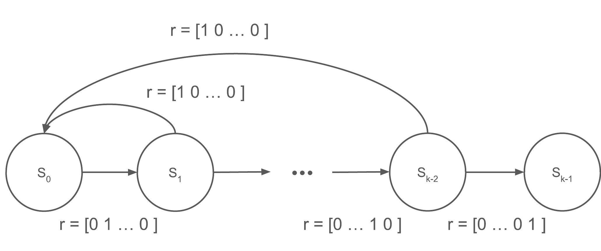
To measure accuracy, we roll out the policy many times from the first state. We compare the returns we collect with the critic's particles. The comparison uses the Wasserstein-2 distance. Lower is better. The bars show medians over 25 random seeds. The error bars are 95% bootstrap confidence intervals.
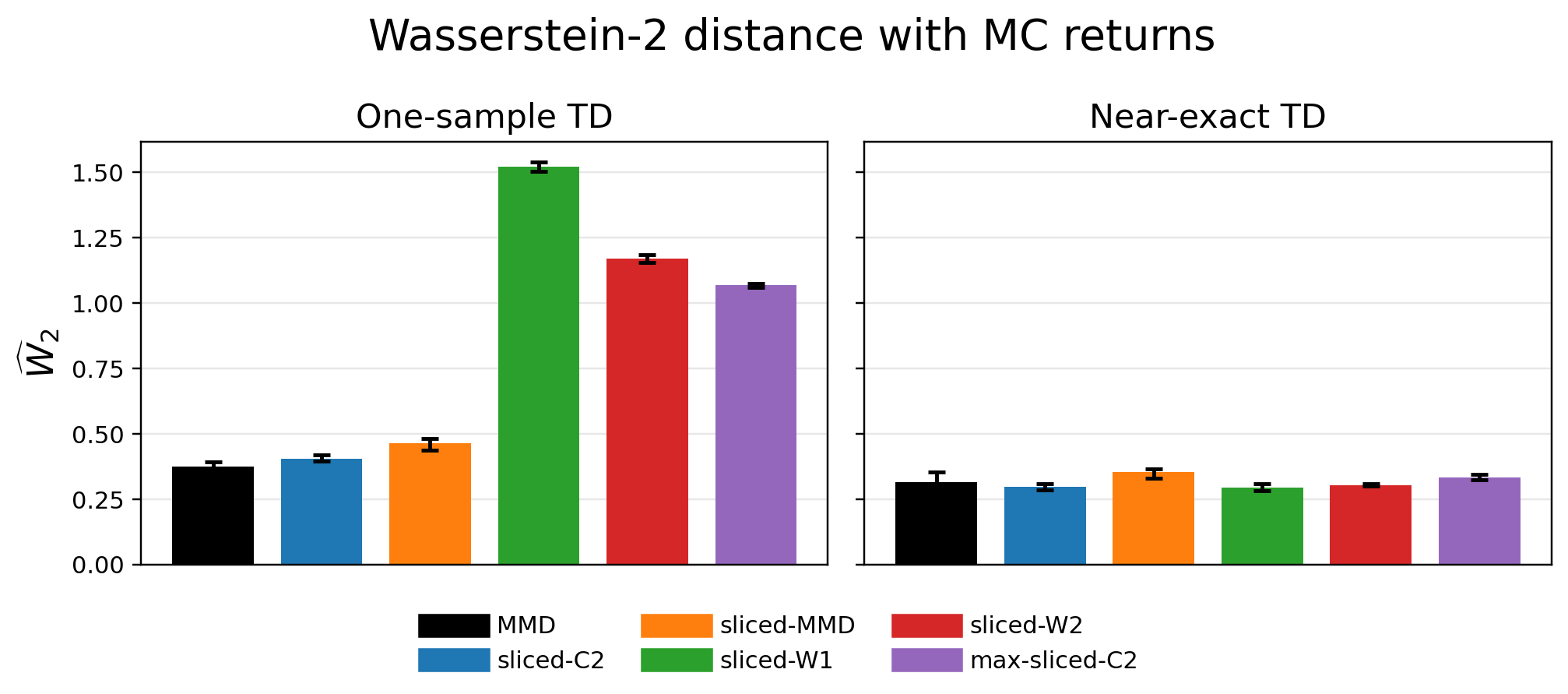
With one-sample TD, sliced Wasserstein and max-sliced Cramér fail to learn the distribution. Their error is two to four times that of the other objectives. With the near-exact update, all six objectives reach about the same error. So these objectives only fail when the target is sampled. This is what the previous section predicts, since their sample gradients are biased.
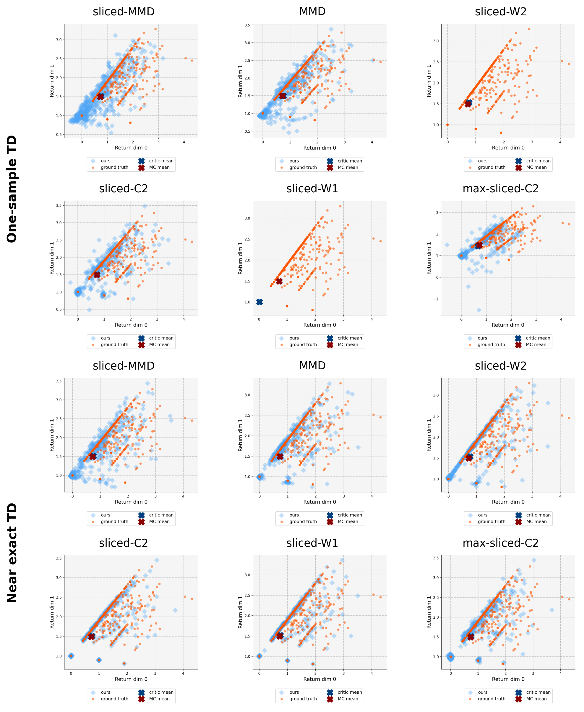
What does failing look like ? The plots below show the returns in orange and the critic's particles in blue, on two return coordinates. The top two rows use one-sample TD and the bottom two the near-exact update. With one-sample TD, the particles of sliced Wasserstein collapse to a single point. For $p=2$, this point sits right on the mean of the returns. Getting the mean right is not the same as learning the distribution.
A maze seen from pixels
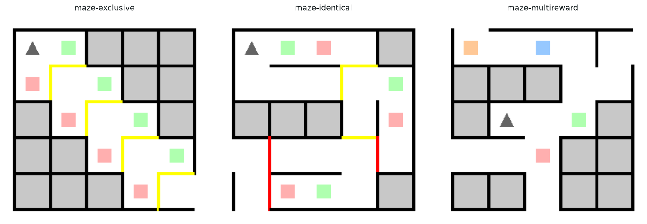
Next, the critic learns from images of a maze [5]. The policy is still fixed and moves at random. Each colored square gives a random reward in the return component of its color. The agent can collect each square once per episode.
Why mazes ? The walls decide which squares the agent can collect in the same episode. Some walls can be crossed in one direction only. In maze-exclusive, the more squares of one color the agent collects, the fewer of the other. In maze-identical, squares of both colors come in pairs. The critic must learn how the return components vary together, not only how large each one is on average.
This time we use plain one-sample TD. Unlike in the chain, we do not build the mixture of possible outcomes. We measure accuracy as in the chain, from the first state. The bars show medians over five random seeds. The error bars are 95% bootstrap confidence intervals.
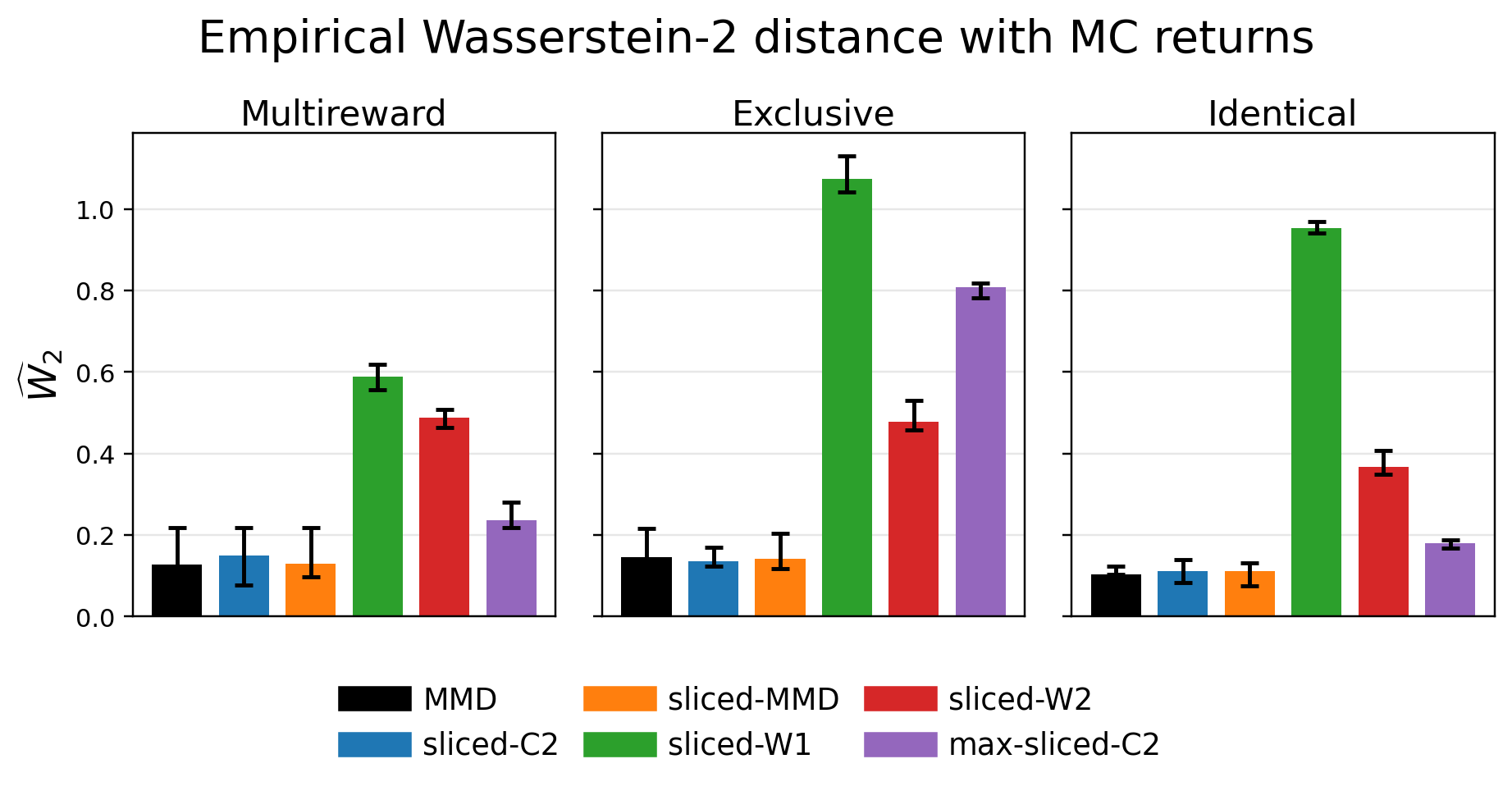
Sliced Cramér, sliced MMD and MMD learn the distributions accurately in all three mazes. Sliced Wasserstein again does poorly, with three to ten times their error. Max-sliced Cramér falls in between, except in maze-exclusive where it fails as well.
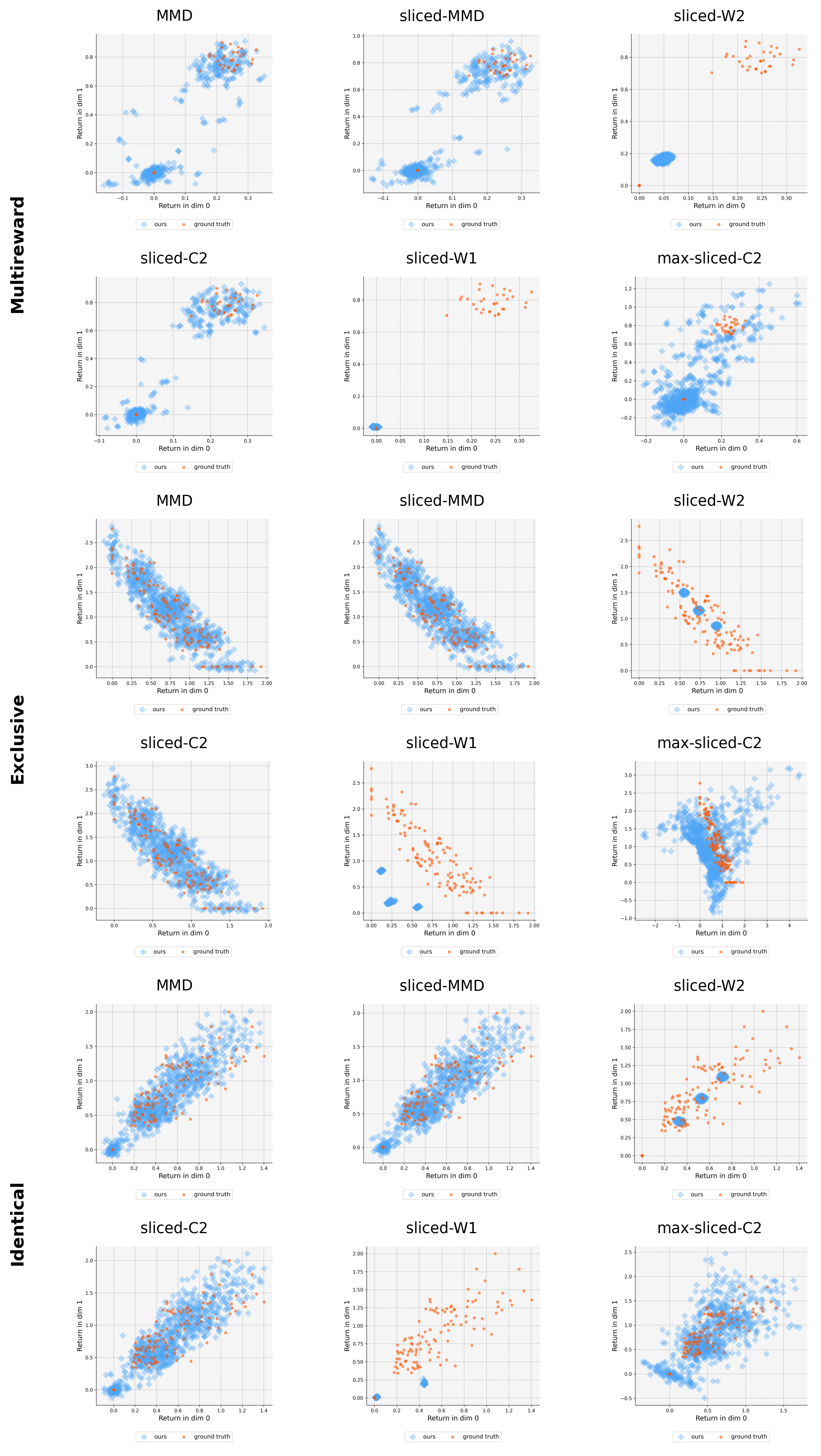
The plots below show what this means. Each maze takes two rows, with two return coordinates. With sliced Cramér, sliced MMD and MMD, the blue particles cover the same regions as the orange returns. In maze-multireward, they even find both groups of returns. Sliced Wasserstein collapses into a few small clumps. Max-sliced Cramér spreads its particles too widely.
Atari games
Our last test is control. The critic now chooses the actions. The agent picks the action with the highest expected return. We use Atari games whose rewards split into several components [5]. The plot shows normalized scores, aggregated over the games. Higher is better.
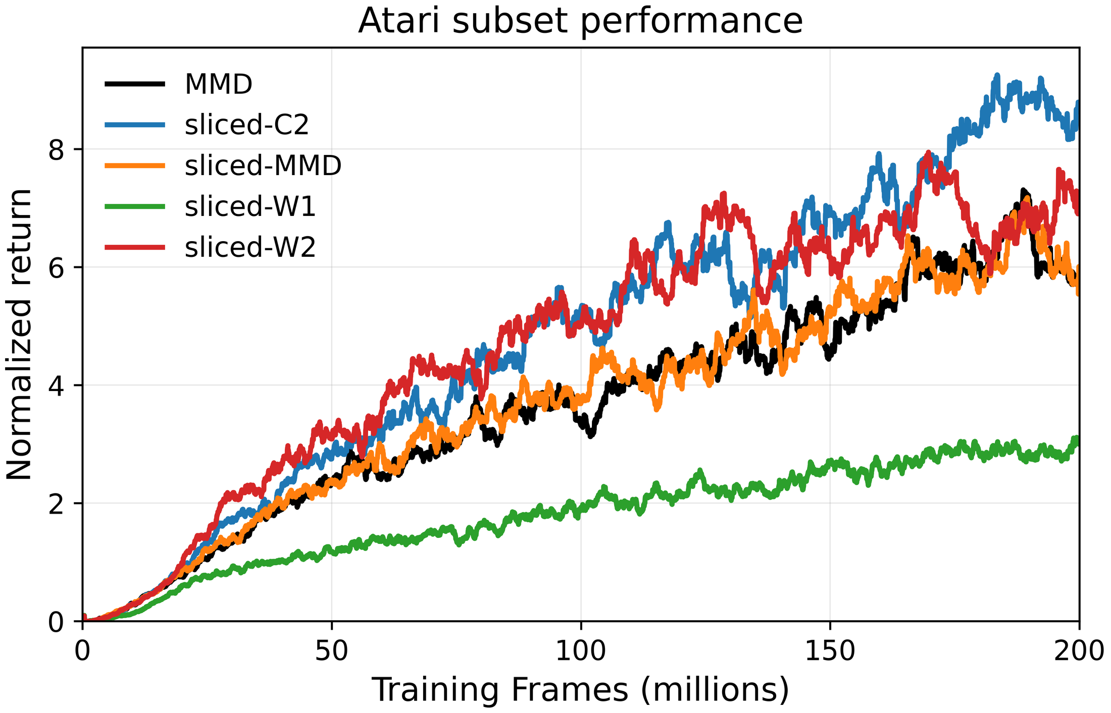
Sliced Cramér scores best. Interestingly, sliced Wasserstein with $p=2$ is not far behind, although it failed to learn the distributions in the chain and the mazes. Only sliced Wasserstein with $p=1$ lags far behind. How can a critic choose good actions without learning the distribution ?
The chain gives the answer. There, sliced Wasserstein collapsed its particles onto the mean of the returns. The mean is all that action selection needs. So a critic can choose good actions while getting the distribution wrong. Good control scores do not show that a critic has learned the return distribution [4].
Practical takeaway
So which objective should you use ? Use sliced Cramér. It learned accurate return distributions in every policy evaluation experiment. It is cheap to compute, and its gradients stay unbiased under one-sample TD.
Sliced MMD is a reasonable alternative. Its kernel gives it more freedom. But in our experiments it brought no clear gain over sliced Cramér. It also costs $\mathcal O(n^2)$ per projection instead of $\mathcal O(n\log n)$.
Avoid sliced Wasserstein and max slicing with one-sample TD. Their gradients are biased, and they failed to learn the distributions in our tests. Good Atari scores do not change this. Action selection only needs the mean. Max slicing does keep a contraction guarantee for general discount matrices. But it picks its direction from the same sampled target, and this biases the gradient.
Open question
None of the objectives we studied has everything we want. Uniform slicing keeps unbiased gradients but loses the contraction bound for general discount matrices. Max slicing keeps the bound but loses unbiased gradients. Can one objective have all of the following ?
- A contraction bound controlled only by the norm of the discount matrix.
- Unbiased gradients for one-sample TD.
- A cheap estimator from samples.
- Estimation error that does not grow sharply with the dimension.
In other words, we are looking for a divergence $\mathcal D$ that satisfies
and remains practical to estimate and optimize from sampled transitions.
Bibliography
- Bellemare, Dabney, and Munos, 2017. A Distributional Perspective on Reinforcement Learning. arXiv.
- Bellemare, Danihelka, Dabney, Mohamed, Lakshminarayanan, Hoyer, and Munos, 2017. The Cramér Distance as a Solution to Biased Wasserstein Gradients. arXiv.
- Dabney, Rowland, Bellemare, and Munos, 2018. Distributional Reinforcement Learning with Quantile Regression. arXiv.
- Rowland, Dadashi, Kumar, Munos, Bellemare, and Dabney, 2019. Statistics and Samples in Distributional Reinforcement Learning. arXiv.
- Zhang, Chen, Zhao, Xiong, Qin, and Liu, 2021. Distributional Reinforcement Learning for Multi-Dimensional Reward Functions. OpenReview.
- Wiltzer, Farebrother, Gretton, and Rowland, 2024. Foundations of Multivariate Distributional Reinforcement Learning. arXiv.
- Rabin, Peyré, Delon, and Bernot, 2011. Wasserstein Barycenter and its Application to Texture Mixing. Springer.
- Bonneel, Rabin, Peyré, and Pfister, 2015. Sliced and Radon Wasserstein Barycenters of Measures. Springer.
- Nadjahi, Durmus, Chizat, Kolouri, Shahrampour, and Simsekli, 2020. Statistical and Topological Properties of Sliced Probability Divergences. arXiv.
- Deshpande et al., 2019. Max-Sliced Wasserstein Distance and Its Use for GANs. arXiv.
- Gretton, Borgwardt, Rasch, Schölkopf, and Smola, 2012. A Kernel Two-Sample Test. JMLR.
- Nguyen-Tang, Gupta, and Venkatesh, 2021. Distributional Reinforcement Learning via Moment Matching. arXiv.
- Killingberg and Langseth, 2023. The Multiquadric Kernel for Moment-Matching Distributional Reinforcement Learning. OpenReview.
- Barreto et al., 2017. Successor Features for Transfer in Reinforcement Learning. arXiv.
- Debes and Tuytelaars, 2026. Distributional Value Gradients for Stochastic Environments. arXiv.
- Hessel, Modayil, van Hasselt, Schaul, Ostrovski, Dabney, Horgan, Piot, Azar, and Silver, 2018. Rainbow: Combining Improvements in Deep Reinforcement Learning. arXiv.
- Felten, Alegre, Nowé, Bazzan, Talbi, Danoy, and da Silva, 2023. A Toolkit for Reliable Benchmarking and Research in Multi-Objective Reinforcement Learning. Proceedings of NeurIPS 2023. OpenReview.
- Fedus, Gelada, Bengio, Bellemare, and Larochelle, 2019. Hyperbolic Discounting and Learning Over Multiple Horizons. arXiv.
- Dabney, Ostrovski, Silver, and Munos, 2018. Implicit Quantile Networks for Distributional Reinforcement Learning. arXiv.
- Fournier and Guillin, 2015. On the Rate of Convergence in Wasserstein Distance of the Empirical Measure. arXiv.
- Debes and Tuytelaars, 2026. Bellman Contraction under MMD: A Unified Framework. arXiv.